ENEE 684 Lecture 9

Overview

Ergun Simsek connects sampling, signal propagation, and optical-fiber dispersion, distinguishing material dispersion from waveguide geometry and showing how their contributions can be engineered to cancel. He then derives the time-domain linear Schrödinger equation from a Taylor expansion of the propagation constant, explaining how β₂ causes pulse broadening and frequency-dependent phase shifts.

Key takeaways

Adding antennas to an inversion system has diminishing returns once the measurements sufficiently sample the recoverable spatial detail; Simsek’s example showed little image improvement beyond roughly 40 antennas.
Material dispersion comes from the wavelength dependence of refractive index, while waveguide dispersion comes from wavelength- and geometry-dependent changes in a mode’s effective index.
Dispersion-shifted fiber balances positive material dispersion against negative waveguide dispersion near a selected wavelength, but the cancellation is limited to a wavelength band.
The dispersion parameter D = −(2πc/λ₀²)β₂ expresses pulse broadening in ps/(nm·km), while β₂ is the coefficient used directly in envelope-propagation equations.
The β₂ term in the linear Schrödinger equation makes pulse frequencies accumulate different phases, producing both temporal broadening and chirp.

Chapters

0:00 Sampling Limits, Antenna Counts, and Phase-Arrival Sensing

A sinusoid needs enough spatial samples to represent its shape; Simsek illustrates this with roughly 20 samples per wavelength.
In an electromagnetic inversion example, increasing the antenna count improved images only up to a point; beyond about 40 antennas, extra measurements brought little benefit.
Differences between phase-front arrival and pulse-energy arrival can support cable-break localization, distance sensing, temperature sensing, and structured-light imaging.

3:25 Sellmeier Models and Material Dispersion in Optical Materials

Sellmeier equations describe the refractive index versus wavelength for low-loss dielectric materials such as fused quartz and sapphire.
Lorentz–Drude-type models are used for lossy optical materials, including gold, silver, and copper in the visible spectrum.
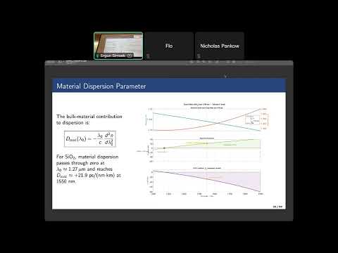
Material dispersion arises because refractive index varies with wavelength; its coefficient depends on the second wavelength derivative of refractive index.

7:10 Dispersion Cancellation and Limits of Epsilon-Near-Zero Materials

Silicon dioxide has a material-dispersion zero near 1.27 μm, while communication systems commonly use wavelengths around 1550 nm.
At 1550 nm, positive material dispersion can potentially be offset by negative waveguide dispersion through suitable geometry.
Epsilon-near-zero materials have a real permittivity near zero but retain loss; strong impedance mismatch and reflection can make coupling difficult.
Thin films can have dielectric responses different from bulk material, so bulk permittivity models may not predict few-layer behavior.

12:00 How Waveguide Geometry Creates Optical Dispersion

A guided mode’s effective index shifts with wavelength because the optical field’s energy distribution between core and cladding changes.
At long wavelengths, more energy can extend into the cladding; at shorter wavelengths, the mode is more concentrated in the core.
Changing waveguide dimensions also changes effective index, producing geometric or waveguide dispersion in addition to material dispersion.

15:00 Estimating Step-Index Fiber Dispersion with V and B

For a step-index fiber, the normalized propagation constant B is calculated from the effective index and the core and cladding indices.
The normalized frequency V depends on fiber radius, wavelength, and numerical aperture; the lecture uses V below about 3 as a single-mode rule of thumb.
Evaluating B and V at several wavelengths allows waveguide dispersion to be estimated; Simsek notes it is negative for the step-index case discussed.

18:00 Dispersion-Shifted Fiber and the Meaning of D

Dispersion-shifted fiber is designed so material and waveguide dispersion cancel near a chosen operating wavelength, such as 1550 nm.
The cancellation generally holds over a limited wavelength band, so fiber specifications identify the wavelength range over which dispersion remains low.
The dispersion parameter D relates to β₂ by D = −(2πc/λ₀²)β₂ and is often reported in ps/(nm·km).
That unit describes pulse broadening in picoseconds per nanometer of spectral width after one kilometer of propagation.

22:00 Finite Differences for a Silicon-Dioxide Dispersion Example

A centered second-difference formula estimates curvature from refractive-index measurements at λ−h, λ, and λ+h.
The estimate is used to calculate material dispersion for bulk silicon dioxide, without adding waveguide dispersion.
The example yields approximately 21.9 ps/(nm·km) for material dispersion and β₂ of about −27.9 ps²/km.

26:00 How β₂ Produces Pulse Broadening and Chirp

Including β₂ in the propagation-constant Taylor expansion makes wavenumber vary quadratically with frequency offset.
Different frequency components then propagate with different phase and group behavior, broadening a narrowband pulse.
In a lossless medium, pulse energy remains conserved as the pulse broadens, so its peak intensity decreases.
Dispersion also adds a frequency-dependent phase, creating chirp; larger |β₂| produces a stronger effect.

33:00 Deriving the Time-Domain Linear Schrödinger Equation

Simsek starts with the frequency-domain envelope and expands β around the carrier frequency, retaining β₀, β₁, and β₂.
The Fourier-domain rule that multiplication by jω corresponds to a time derivative converts frequency powers into temporal derivatives.
Changing to retarded time, which accounts for propagation at the group velocity, removes the first-order time-derivative term.
The resulting envelope equation relates the spatial derivative to the second time derivative, scaled by β₂; Simsek also checks that both sides have units of inverse meters.

43:00 Interpreting the Envelope Equation and Previewing MATLAB Waveguide Analysis

The equation predicts that propagation accumulates a phase proportional to the square of the frequency offset, alongside pulse broadening.
Strong chirp can shift optical frequencies away from a receiver’s narrow detection band, creating a communication-system limitation.
Simsek postpones the Gaussian-pulse solution to the next lecture and previews MATLAB calculations of effective index and waveguide dispersion.

Summary, takeaways, and chapters were generated by AI from the video's transcript and may contain errors. The video belongs to its creator, Ergun Simsek.