ENEE 684 Introduction to Photonics, Lecture 12 Dielectric Waveguides (Part 2)

Overview

Ergun Simsek develops a 2D mode-expansion method for estimating dielectric-waveguide taper transmission, using normalized mode profiles, interface overlap integrals, propagation phases, and S-matrix star products. The lecture applies the method to adiabatic tapers, inverse-taper design, and grating couplers, emphasizing practical coupling losses from reflection and alignment as well as checks against 3D FDTD results.

Key takeaways

A 2D mode-expansion model can estimate long-taper transmission efficiently by combining normalized interface modes, overlap-derived S-matrices, propagation phases, and star products that account for repeated internal reflections.
A roughly 1-micrometer chip waveguide coupled directly to a roughly 10-micrometer fiber output can incur about 20 dB of loss, so mode-size matching with lenses, gratings, or tapers is essential.
Taper length and sampling density both matter: the lecture's example approaches stable efficiency around 50 micrometers, while roughly 100 samples across a 100-micrometer linear taper provide a useful starting point.
The demonstrated mode-expansion result of about 95% transmission is close to a 93.9% 3D FDTD result, supporting its use for fast design exploration before final full-wave validation.
For the cited inverse-taper comparison, a quadratic width profile outperforms linear and exponential profiles, reaching about 0.4 dB minimum loss; the best geometry remains dependent on wavelength and fabrication constraints.
Coupling efficiency must include more than taper transmission: laser-mode overlap, facet reflection, and XYZ alignment each contribute losses that multiply into the system-level result.

Chapters

0:00 Adjoint Optimization and the Mode-Expansion Goal

The adjoint example begins with a point source and randomly assigned permittivity in each design pixel, then uses forward and reciprocal simulations to update the structure.
A small update coefficient, such as 10^-4, can gradually shape the design toward a target such as maximizing electric field.
The lecture shifts to mode expansion, a method used in commercial solvers including Ansys Lumerical and Tidy3D, to analyze waveguide tapers.

3:40 Fiber-to-Chip Size Mismatch and Why Tapers Matter

A typical chip waveguide is about 1 micrometer wide, while a cleaved fiber output can be around 10 micrometers across.
Without a coupling structure, the size mismatch can produce roughly 20 dB of loss; a lensed fiber can focus a 10-micrometer spot toward 2 micrometers.
Tapers also support mode conversion, power splitting, and connections to lasers, amplifiers, and modulators.

8:00 Adiabatic Tapers Preserve Light During Width Changes

A taper changes waveguide width gradually over a length commonly ranging from about 100 to 500 micrometers.
An adiabatic transition changes the geometry slowly enough that the optical field can transfer into the desired waveguide mode with limited radiation loss.
At a wavelength near 1 micrometer, a 200-micrometer taper spans about 200 wavelengths, making a full 3D simulation computationally demanding.

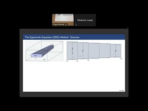
11:00 Discretizing the Taper into Mode-Profile Interfaces

The taper is divided into N sections, producing N+1 interfaces with progressively changing waveguide widths.
A 2D solver computes electric- and magnetic-field profiles at each interface; the profiles are normalized using the integrated power over the computational domain.
A practical multimode calculation should retain roughly four or five modes, although the lecture first derives the simpler fundamental-mode case.

13:45 How Waveguide Width Changes Effective Index and Field

Simsek's MATLAB example shows that narrowing the waveguide lowers its effective index and increases the normalized electric-field amplitude.
The stored interface data include transverse electric and magnetic field components and the effective indices needed to calculate propagation constants.
Field intensification in a narrower guide can matter for high-energy lasers, where increased electric fields may either be useful or risk ionization.

17:40 Overlap Integrals and Propagation Phases Build the Model

The method computes interface overlap integrals from the electric field on one interface and magnetic field on the neighboring interface, and vice versa.
These overlaps form reflection and transmission terms analogous to microwave S-parameters such as S11 and S21.
Propagation through section i adds phase factors based on its length and propagation constant; material loss can add amplitude decay as well.

24:40 S-Matrix Star Products Account for Repeated Reflections

Adjacent interface matrices and propagation matrices are combined to relate incoming amplitudes to outgoing amplitudes.
The star-product algebra removes internal wave amplitudes while accounting for the infinite series of reflections between interfaces.
For the assembled taper, the transmission and reflection terms yield power efficiencies; in the lossless model, untransmitted power is attributed to mode-conversion or radiation loss.

30:40 Sampling Density, Taper Length, and FDTD Validation

The interface spacing must be small enough for the geometry to change adiabatically; the lecture relates the spacing to the width-change rate and overlap between neighboring modes.
A linearly varying taper about 100 micrometers long can be represented with roughly 100 samples as an initial rule of thumb.
One example gives approximately 95% transmission from mode expansion, compared with 93.9% from a 3D FDTD calculation, indicating close agreement.
Increasing taper length from 1 to 100 micrometers raises calculated coupling efficiency; the example is nearly stable by about 50 micrometers for a loss target below 0.5 dB.

34:00 Grating Couplers Trade Polarization and Bandwidth for Access

A grating coupler uses a periodic structure and angled illumination to redirect light into a chip waveguide.
Its period and input polarization are critical; the described configuration works for a specific polarization orientation.
Changing grating periodicity can broaden the operating bandwidth, usually at the cost of lower coupling efficiency.

37:00 Inverse-Taper Profiles: Linear, Quadratic, and Exponential

An inverse taper begins with a very narrow waveguide tip—about 80 to 100 nanometers at a 1550-nanometer wavelength—and widens along the propagation direction.
The lecture compares linear, quadratic, and exponential width profiles; the quadratic design performs best in the cited example, with minimum loss around 0.4 dB.
Longer inverse tapers improve transmission: the cited 100-micrometer design reaches about -0.6 dB, while fabrication imperfections and broken symmetry can affect real devices.

44:00 Fiber Alignment and the Full Coupling-Efficiency Budget

Fiber coupling depends on end-face type, lens-to-chip distance, and XYZ alignment; even a well-designed taper cannot compensate for every positioning error.
A total efficiency estimate multiplies separate factors for laser-to-input mode overlap, facet reflection, alignment, and taper transmission.
The lecture illustrates that mode overlap might be 0.9 and that an air-to-silicon interface reflects a substantial fraction of incident power without index matching.
Lensed fibers and polymer materials can improve focusing and refractive-index matching, reducing losses compared with an untreated interface.

51:00 Coupler Tradeoffs, Solver Limits, and Course Wrap-Up

Grating couplers are relatively tolerant of positional misalignment but are more polarization-sensitive and generally narrower-band than inverse tapers.
Inverse tapers can offer broader bandwidth but demand more advanced fabrication and careful fiber orientation.
Mode expansion is a fast 2D design tool; Simsek recommends verifying the final design with a 3D simulation such as Tidy3D or Ansys Lumerical FDTD.
The closing discussion previews directional couplers, Y-branches, Mach–Zehnder interferometers, circulators, and fiber Bragg gratings, and notes that midterm materials will include formulas and calculation practice.

Summary, takeaways, and chapters were generated by AI from the video's transcript and may contain errors. The video belongs to its creator, Ergun Simsek.