EEL4514C Communication Systems and Components, Fall 2026, Lecture 12

Overview

Mingyue Ji develops the relationship between time-domain autocorrelation and frequency-domain spectral density: for energy signals, the Fourier transform of autocorrelation is the energy spectral density (ESD), while the Wiener–Khinchin theorem extends that connection to power signals and power spectral density (PSD). The lecture derives PSD through time truncation, explains how to calculate power within a frequency band, and works through a periodic unipolar square wave with period T_b and 50% duty cycle, whose PSD consists of weighted impulses at harmonics.

Key takeaways

For an energy signal, autocorrelation and ESD form a Fourier-transform pair: R_g(τ) transforms to |G(f)|².
For a power signal, the Wiener–Khinchin theorem gives the corresponding relationship: PSD is the Fourier transform of long-time-averaged autocorrelation.
PSD provides a direct way to compute average power, and integrating it over a frequency interval gives the power in that band.
A periodic signal has a line-spectrum PSD: impulses occur at its harmonics, with weights equal to the squared magnitudes of its Fourier-series coefficients.
For the amplitude-1 unipolar square wave with period T_b and 50% duty cycle, the DC PSD weight is 1/4, nonzero odd-harmonic weights decay as 1/(π²n²), and nonzero even harmonics vanish.

Chapters

0:00 From Parseval’s Theorem to Energy Spectral Density

The lecture reviews computing signal energy or power in the frequency domain rather than directly in time.
Parseval’s theorem preserves inner products between time and frequency domains; energy and power follow as special cases.
Energy spectral density (ESD) for an energy signal is the squared magnitude of its Fourier transform.

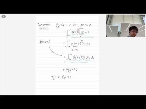
5:25 Autocorrelation Symmetry for Real Energy Signals

Autocorrelation compares a signal with a delayed version of itself using an inner product.
For a real signal g(t), changing the integration variable shows that its autocorrelation is even: R_g(τ) = R_g(−τ).
The delay τ remains fixed while the integration variable is a dummy variable.

10:15 Autocorrelation as Convolution and the ESD Transform Pair

Autocorrelation can be expressed as convolution of g(t) with its time-reversed version g(−t), with conjugation for complex signals.
The Fourier transform of that convolution is G(f)G*(f) = |G(f)|².
Therefore, the Fourier transform of energy-signal autocorrelation is its ESD, and the inverse transform recovers autocorrelation.

15:57 Defining PSD by Truncating a Power Signal

Mingyue Ji turns a power signal into a finite-energy signal by restricting it to the interval from −T/2 to T/2.
The truncated signal’s ESD is normalized by T, and the limit as T approaches infinity defines the power spectral density.
This definition is theoretically useful but often difficult to calculate directly because it requires a Fourier transform and an infinite-duration limit.

22:50 Using PSD to Measure Total and Band-Limited Power

Integrating PSD across frequency yields the signal’s average power.
For a real signal, positive- and negative-frequency contributions are symmetric, so total power can be found by doubling the integral over positive frequencies.
Power passed by a band-pass system can be calculated by integrating PSD only between the band edges f₁ and f₂.

27:47 Wiener–Khinchin Links Power Autocorrelation and PSD

For a power signal, autocorrelation is defined as the long-time average of g(t)g*(t−τ) over a T-length interval.
The Fourier transform of power-signal autocorrelation equals PSD, providing the Wiener–Khinchin theorem.
Although commonly applied to random processes, the lecture first treats g(t) as deterministic.

31:27 Setting Up Autocorrelation for a Periodic Signal

For a periodic signal with period T₀, the long-time autocorrelation integral is divided into successive periods.
The derivation uses the Fourier-series expansion of g(t) and averages across 2N periods as N grows.
This setup converts the time-average calculation into a sum involving the signal’s Fourier-series coefficients.

35:42 Periodic-Signal Autocorrelation from Fourier Coefficients

Integrating the Fourier-series terms over one period produces coefficient products c_m c*_m.
The average over repeated periods removes cross terms, leaving harmonic terms weighted by |c_m|².
The resulting autocorrelation is itself a Fourier series, making its Fourier transform a discrete line spectrum.

41:27 Periodic PSD as Impulses at Harmonic Frequencies

Fourier-transforming the periodic autocorrelation turns each complex exponential into a Dirac delta.
The PSD is a weighted impulse train at integer multiples of the fundamental frequency 1/T₀.
Each harmonic’s impulse weight is the squared magnitude of its Fourier-series coefficient, |c_m|².

44:27 PSD of a 50%-Duty-Cycle Unipolar Square Wave

The example uses a unipolar square wave of amplitude 1, period T_b, and pulse width T_b/2.
Fourier-series coefficients are obtained from the pulse’s Fourier transform using c_n = (1/T_b)G(n/T_b).
The coefficient magnitudes are |c₀|² = 1/4, |c_n|² = 1/(π²n²) for odd n, and zero for nonzero even n.
Its PSD is a discrete set of impulses at f = n/T_b, weighted by those coefficient magnitudes.

Summary, takeaways, and chapters were generated by AI from the video's transcript and may contain errors. The video belongs to its creator, Mingyue Ji.