EEL4514C Communication Systems and Components, Fall 2026, Lecture 09

Overview

Mingyue Ji connects Fourier series coefficients to the Fourier transform of periodic signals: a periodic signal’s spectrum is an impulse train whose weights are its Fourier series coefficients. The lecture applies this result to rectangular pulses and impulse trains, defines first-null and null-to-null bandwidth, shows how cosine modulation shifts spectra, and derives the time-scaling property.

Key takeaways

A periodic signal with Fourier-series coefficients Sₙ and fundamental frequency f₀ has Fourier transform ΣₙSₙδ(f − nf₀), so its spectrum consists of weighted impulses at harmonics.
The periodic impulse train Σₖδ(t − kT₀) transforms to (1/T₀)Σₙδ(f − n/T₀), making impulse trains a central model for sampling in digital communications.
A rectangular pulse of duration τ has first spectral nulls at ±1/τ; the lecture’s one-sided baseband first-null bandwidth is therefore 1/τ.
Cosine modulation by a carrier at fc shifts the spectrum to ±fc; the positive-frequency rectangular-pulse lobe spans 2/τ between its first nulls.
Time scaling creates an inverse frequency scaling: shortening a pulse supports faster transmission but broadens its spectrum, while widening it narrows the spectrum.

Chapters

0:00 Review: Computing Fourier Series Coefficients from the Fourier Transform

The previous lecture related a periodic signal’s Fourier series coefficients to the Fourier transform of one nonperiodic period.
For fundamental period T₀ and frequency f₀ = 1/T₀, the relationship is Sₙ = (1/T₀)G(n/T₀) = f₀G(nf₀).
Mingyue Ji previews periodic-signal transforms, bandwidth, and further Fourier-transform properties; Lab 2 is also announced.

5:25 The Delta Function Sampling Property and the Exponential Transform Pair

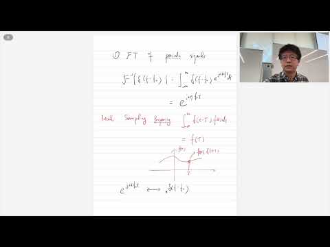
The sampling property evaluates an integrand at the location of a delta function: integrating g(f)δ(f − f₀) gives g(f₀).
Applying that property to the inverse Fourier transform gives the pair e^(j2πf₀t) ↔ δ(f − f₀).
This pair makes it possible to represent periodic time-domain signals in the Fourier-transform domain.

9:30 Deriving the Fourier Transform of a Periodic Signal

Write a periodic signal as its Fourier series, S(t) = Σₙ Sₙe^(j2πnf₀t).
Linearity lets the Fourier-transform operator act on each complex exponential separately.
The resulting spectrum is S(f) = Σₙ Sₙδ(f − nf₀): impulses at harmonics nf₀, weighted by Fourier series coefficients Sₙ.

12:17 Rectangular Pulse Trains: Sampling the Sinc Spectrum

A single rectangular pulse has a sinc-shaped Fourier transform, and the periodic pulse train’s Fourier series samples that spectrum at integer multiples of f₀.
Each sampled value becomes the weight of a delta impulse in the periodic signal’s Fourier transform.
The first sinc zero occurs at 1/τ for pulse duration τ, locating the first nulls of the sampled spectrum.

16:00 When Pulse Duration Equals Period, the Pulse Train Becomes Constant

When τ = T₀, adjacent rectangular pulses meet with no gaps, producing a constant time-domain signal.
The Fourier-series samples at nonzero harmonics fall on sinc zero crossings, leaving only the DC component.
The Fourier transform is therefore a single delta impulse at zero frequency, consistent with the transform of a constant.

19:42 Impulse Trains Transform into Impulse Trains

For a periodic train of unit impulses spaced by T₀, the Fourier-series coefficient integral uses the delta sampling property and gives Sₙ = 1/T₀ for every n.
Its Fourier transform is another impulse train: (1/T₀)Σₙδ(f − n/T₀).
This time–frequency duality matters in digital communications: multiplying a continuous-time signal by an impulse train samples it, while the frequency-domain operation is convolution with a frequency-domain impulse train.

31:56 First-Null Bandwidth of a Baseband Square Pulse

Bandwidth has multiple definitions; one useful measure is the frequency span retained around the signal’s main lobe.
For a baseband rectangular pulse of duration τ, the sinc spectrum’s first zeros lie at ±1/τ.
The lecture calls the one-sided span from zero to the first null the first-null bandwidth, B = 1/τ.

36:20 Cosine Modulation Shifts the Sinc Spectrum and Doubles Null-to-Null Width

Modulating g(t) by cos(2πfct) creates two frequency-shifted copies of G(f), centered at +fc and −fc, each scaled by one half.
For a rectangular pulse, the positive-frequency lobe’s first nulls are at fc − 1/τ and fc + 1/τ, giving null-to-null bandwidth 2/τ.
The shift moves the baseband spectrum to a carrier band; the negative-frequency copy of a real signal does not represent additional independent information.

43:34 Time Scaling Trades Pulse Duration for Frequency Spread

Starting from the Fourier-transform definition and substituting u = at derives the time-scaling relationship.
For a > 0, g(at) transforms to (1/a)G(f/a); more generally, the scale factor is 1/|a|.
Widening a signal in time narrows its frequency spectrum, while shrinking a pulse to transmit symbols faster spreads its spectrum.

Summary, takeaways, and chapters were generated by AI from the video's transcript and may contain errors. The video belongs to its creator, Mingyue Ji.