EEL4514C Communication Systems and Components, Fall 2026, Lecture 05

Overview

Mingyue Ji reviews communication-loss calculations and decibel power units, then builds foundations for continuous-time signal analysis: complex-number representations, inner products, signal energy and average power, DC values, and special functions. The lecture connects Fourier-series and transform choices to signal periodicity, explains why complex exponentials are central to frequency analysis, and introduces continuous-time Dirac and discrete-time Kronecker delta functions.

Key takeaways

A 10× increase in propagation distance produces a 20 dB power loss in the reviewed path-loss model, while doubling distance produces a 6 dB loss.
Power references determine the absolute decibel unit: dBm uses 1 mW, dBW uses 1 W, and their values differ by 30 dB.
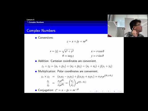
Cartesian complex numbers simplify addition, whereas polar form simplifies multiplication and division; phase calculations must account for the correct quadrant.
Fourier series target periodic signals, Fourier transforms extend frequency analysis to nonperiodic signals, and Laplace transforms handle cases where the Fourier transform does not converge.
A finite-energy signal has zero long-term average power, so energy and power signals are distinguished by requiring positive finite energy or positive finite average power, respectively.
The continuous-time Dirac delta and discrete-time Kronecker delta both have unit total weight, but the former is a continuous-time idealization while the latter is an ordinary sequence with value 1 at n = 0.

Chapters

0:00 Lab 1 Logistics and Review of Path Loss and Decibel Power

Lab 1 covers Fourier series, is scheduled to run for two weeks, and is due the following Friday.
Received power at distance d is calculated from power at a reference distance d₀ and the path-loss factor.
In the reviewed path-loss model, doubling distance corresponds to a 6 dB power loss; increasing distance tenfold corresponds to 20 dB.
Power in dBm is referenced to 1 mW, power in dBW to 1 W, and dBm = dBW + 30; Voyager 2 and CDMA are mentioned as examples.

4:50 Why Fourier Series, Fourier Transforms, and Laplace Transforms Differ

Fourier series were introduced to analyze periodic signals by decomposing them into frequency components.
Fourier transforms extend frequency analysis to nonperiodic signals, and can also represent periodic signals using delta functions.
Some signals do not have a convergent Fourier transform; the Laplace transform addresses broader cases using a region of convergence.
The course will also distinguish continuous-time tools from discrete-time methods such as the DFT and Z-transform.

9:30 Complex Numbers: Cartesian and Polar Forms for Communication Signals

A complex number z = x + jy has real component x, imaginary component y, and imaginary unit j = √−1.
In communications, the real and imaginary components are commonly called the in-phase and quadrature components.
Polar form z = |z|e^(jθ) uses magnitude √(x² + y²); Cartesian form is convenient for addition, while polar form simplifies multiplication and division.
The phase is conventionally represented in the range −π to π; arctan(y/x) alone can give the wrong quadrant, so the angle must be adjusted or computed with quadrant awareness.

16:00 Complex Conjugates and Euler’s Formula

Complex conjugation changes the sign of the imaginary component in Cartesian form and the sign of the phase in polar form.
Euler’s formula, e^(jθ) = cos θ + j sin θ, yields cosine and sine as combinations of positive- and negative-frequency complex exponentials.
The lecture motivates Euler’s formula through Taylor expansions and identifies it as a foundation of frequency-domain analysis.
Every e^(jθ) has magnitude 1, so varying θ traces the unit circle in the complex plane.

19:15 Inner Products, L2 Norms, and Orthogonality

For continuous-time functions, the inner product integrates f(t)g*(t) over the real line; for complex vectors, the corresponding operation is a sum.
Setting the two arguments equal gives the squared L2 norm, using |f(t)|² or the sum of squared vector magnitudes.
Two functions or vectors are orthogonal when their inner product is zero.
These definitions provide tools for comparing signals and will be used later in the course.

21:20 Energy Signals: Finite Total Squared Magnitude

Signal energy is the integral of |g(t)|² over all time; a nonzero signal with finite energy is classified as an energy signal.
A finite-amplitude, finite-duration square pulse is an energy signal because its total squared magnitude integrates to a finite value.
Finite duration and finite amplitude are sufficient but not necessary: a decaying exponential can last forever and still have finite energy.
A signal can also become unbounded near a point yet have finite energy if the integral of its squared magnitude remains finite.

26:20 Average Power, Periodicity, and the Energy–Power Distinction

Average power is the limit, as T grows without bound, of the signal energy over a length-T interval divided by T.
For a periodic signal, power can be computed over one period as the integral of |g(t)|² divided by the period; the fundamental period is the smallest repeat interval.
A nonzero energy signal has zero long-term average power, so the power-signal definition requires finite, strictly positive average power.
Periodic sinusoids are power signals; long practical waveforms can often be approximated as periodic because they contain many cycles.

36:15 DC Component as the Long-Term Signal Average

The DC component is the signal’s long-term average, computed by integrating over a symmetric interval and dividing by its duration as that duration approaches infinity.
A constant offset carries no changing information but consumes transmission power, so communication systems often aim for zero DC.
Some practical systems retain a nonzero DC component because it can make receiver operation easier.

38:20 Complex Exponential Signals: Period, Power, and Causality

The function e^(jωt) has unit magnitude, phase ωt modulo 2π, and fundamental period 2π/ω.
Because it is periodic and persists over time, a nonzero complex exponential is a power signal rather than an energy signal.
A causal signal is zero for t < 0; an anti-causal signal is zero for t ≥ 0, while a signal nonzero on both sides of zero is noncausal.
Euler’s formula converts cosine and sine into complex exponentials, and e^(jπ) = −1 gives the useful identity (−1)^n = e^(jnπ).

44:25 Dirac and Kronecker Delta Functions and Delta Weighting

The continuous-time Dirac delta is zero away from t = 0 and is defined by having unit integral; it is a mathematical idealization of a very narrow, high-amplitude pulse with area 1.
The discrete-time Kronecker delta equals 1 at integer n = 0 and 0 at every other integer, so its sum over all integers is 1.
Scaling a continuous-time delta by C scales its integral to C; multiplying g(t) by δ(t) selects g(0), and δ(t − T) selects g(T).
The lecture begins the delta-function sampling property and leaves its further explanation for the next lecture.

Summary, takeaways, and chapters were generated by AI from the video's transcript and may contain errors. The video belongs to its creator, Mingyue Ji.