EEL4514C Communication Systems and Components, Fall 2026, Lecture 04

Overview

Mingyue Ji develops practical link-budget calculations from free-space propagation: received power falls as distance squared and, for fixed antenna gains, as frequency squared; a reference-distance model expresses additional path loss in decibels. The lecture also distinguishes dB ratios from absolute power levels in dBW and dBm, then applies the free-space equation to a 1,897 MHz CDMA link, obtaining approximately 3.2 × 10⁻⁵ W, or −45 dBW (−15 dBm), at 100 m.

Key takeaways

For free-space propagation, received power varies as 1/d², so doubling distance adds about 6 dB of path loss and a tenfold distance increase adds 20 dB.
A reference-distance model computes received power by subtracting PL(dB) = 10nlog₁₀(D/D₀) from the received power at D₀; free space uses n = 2.
dBW and dBm are absolute power levels referenced to 1 W and 1 mW, respectively, so dBm = dBW + 30 for the same power.
Using a 1 m reference distance, Voyager 2’s approximate 19.5-billion-kilometer distance corresponds to about 266 dB of free-space distance loss.
A 1,897 MHz link with 17 dBi transmit gain, 3 dBi receive gain, and 13 dBW transmit power yields about 3.2 × 10⁻⁵ W (−15 dBm) at 100 m under the Friis model.
Real wireless links can depart from free space because obstacles, distance-dependent path-loss exponents, shadowing, and fading alter received power; 3GPP-style models capture more practical conditions.

Chapters

0:00 Free-Space Propagation, Antenna Gain, and Path-Loss Recap

An isotropic radiator spreads transmit power over a sphere of area 4πd², giving power density PT/(4πd²) at distance d.
Transmit gain GT and receive effective aperture AE connect power density to received power; AE = GRλ²/(4π) yields the Friis free-space equation.
The free-space model predicts received power proportional to 1/d² and 1/f²; real obstacles can make distance decay steeper.
Power ratios use dB = 10log₁₀(ratio): 2× is about 3 dB, 5× about 7 dB, and 10× exactly 10 dB; dBi and dBd specify antenna-gain references.

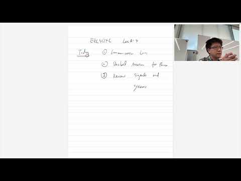
8:00 Lecture 04 Goals: Reference-Distance Loss and Signal-Systems Review

The lecture finishes communication-loss modeling, introduces dBW and dBm, and begins a planned two- or three-lecture review of continuous-time signal systems.
Mingyue Ji frames communication engineering as an application of signal-and-systems tools for designing and analyzing communication systems.
The review leads into large-scale propagation models that use a known received-power value at a reference distance.

10:20 Large-Scale Propagation Models Start from a Known Reference Point

A close-in reference distance D₀ provides a baseline received power, PR(D₀), so power at another distance can be found by applying the additional path loss.
PR(D₀) can be obtained by measurement or estimated with the Friis equation when free-space conditions are a reasonable approximation.
The Friis equation applies in the far field, where the wavefront and phase are approximately consistent across the receiving antenna aperture.

14:00 Far-Field Assumptions and the Distance Dependence of Path Loss

A nearby transmitter can produce substantial phase differences across a large antenna, unlike a distant source whose incident wave is more nearly uniform across the aperture.
For fixed antenna size, the far-field distance increases with frequency; the Friis estimate remains useful for many cellular and Wi-Fi links.
Mingyue Ji notes that practical propagation models account for obstacles and may use different distance exponents in different regions.

17:20 Deriving Relative Path Loss from the Reference-Distance Power

In free space, the ratio of received powers at D₀ and D is PR(D)/PR(D₀) = (D₀/D)².
Taking the power ratio in dB gives a positive loss PL(dB) = 20log₁₀(D/D₀), and received power becomes PR(D₀) in dB minus PL.
For a more general path-loss exponent n, distance-dependent loss is 10nlog₁₀(D/D₀); free space has n = 2.

22:00 Distance-Doubling Rules and Voyager 2’s 266 dB Path Loss

With free-space distance exponent 2, doubling distance multiplies path loss by four, adding about 6 dB; increasing distance tenfold adds 20 dB.
For Voyager 2 at approximately 19.5 billion kilometers from Earth, using D₀ = 1 m gives 20log₁₀(19.5 × 10¹²) ≈ 266 dB.
That 266 dB loss corresponds to a linear ratio of roughly 3.8 × 10²⁶; converting dB back to a power ratio still uses division by 10.

33:00 Absolute Power Levels: Converting Between Watts, dBW, and dBm

Linear transmit power is commonly specified in watts or milliwatts, with 1 W = 1,000 mW.
dBW uses 1 W as its reference: power in dBW is 10log₁₀(power in watts); dBm uses 1 mW and 10log₁₀(power in milliwatts).
Because 1 W equals 1,000 mW, the same power’s dBm value is its dBW value plus 30 dB.
A phone’s transmit power is described as typically around 20 dBm, illustrating why dBm is a common practical power unit.

39:30 Setting Up a 1,897 MHz CDMA Base-Station Link Budget

The worked example uses a CDMA (code division multiple access) base station transmitting at 1,897 MHz and asks for received power at 100 m.
The link includes a directional transmit antenna with 17 dBi gain and a receive antenna with 3 dBi gain; dBi expresses gain relative to an isotropic radiator.
The calculation uses free-space propagation and does not add a separate concrete-penetration factor; more detailed standards and models account for environmental effects.
Mingyue Ji notes that practical propagation models may vary the path-loss exponent by distance and can include shadowing and fading.

46:00 Free-Space Link-Budget Result and the Next Signal-Systems Review

For the worked calculation, the transmitted power is converted as 13 dBW ≈ 20 W; antenna gains convert to linear factors of 50 and 2.
At 1,897 MHz, the wavelength is approximately 0.158 m; substituting it and the 100 m distance into Friis gives about 3.2 × 10⁻⁵ W.
The received level is approximately −45 dBW, or −15 dBm after adding 30 dB.
The next lecture begins the planned review of signal systems.

Summary, takeaways, and chapters were generated by AI from the video's transcript and may contain errors. The video belongs to its creator, Mingyue Ji.