EEL4514C Communication Systems and Components, Fall 2026, Lecture 03
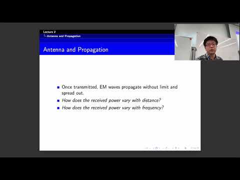 Watch on YouTube →
Overview
Mingyue Ji connects electromagnetic-wave propagation to practical link-budget calculations, deriving wavelength from propagation delay and introducing the Friis free-space equation for received power. The lecture then shows how distance and frequency affect received power, explains dB, dBi, and dBd conversions, and derives a free-space path-loss formula with an adjustable distance exponent for non-ideal environments.
Key takeaways
- Wavelength is λ = c/f: a 900 MHz signal has a wavelength of about 0.33 m, while a 1 MHz signal is about 300 m, affecting practical antenna size.
- The Friis free-space equation, P_R = P_TG_TG_R(λ/(4πD))², combines transmit gain, receive gain, wavelength, and separation to estimate received power.
- For fixed antenna gains in free space, received power falls as 1/D² and 1/f²; higher frequencies therefore generally require shorter links or other compensating measures.
- A power gain of 3 dB is approximately a factor of 2, 7 dB is about a factor of 5, and 10 dB is a factor of 10; convert using G_dB = 10log₁₀(G).
- Antenna gain references matter: dBi compares with an isotropic radiator, while dBd compares with a half-wave dipole, which is approximately 2.15 dBi.
- Free-space path loss in SI units is approximately 20log₁₀(f) + 20log₁₀(D) − 147.6 dB; real environments can raise the distance exponent above 2.
Chapters
0:00
Course Logistics and Review of Frequency, Light Speed, and Propagation
- Mingyue Ji says Lab 1 should be uploaded soon so students who finished Lab 0 can continue.
- The review emphasizes the speed of light, approximately 3 × 10^8 m/s, and SI prefixes such as kilo, mega, and giga.
- Wi-Fi devices commonly operate in the 2.4 GHz and 5 GHz bands, illustrating how frequency is specified in communications.
1:35
Voyager Signals: Long Distances, Low Transmit Power, and Earth Antennas
- A radio message takes roughly 23–24 hours to travel from Earth to Voyager 1, illustrating the vast distance involved.
- Ji cites Voyager's transmit power as about 22 W and notes that its power comes from a nuclear source as sunlight becomes unavailable.
- The Deep Space Network uses antennas at three locations, including the United States, Australia, and Spain, to maintain coverage as Earth rotates.
6:36
Wavelength Derivation and Surface Effects on Radio Propagation
- Starting with a cosine signal and delay τ = D/c, Ji derives wavelength as λ = c/f, or equivalently λ = 2πc/ω.
- At 900 MHz, wavelength is about 0.33 m; at 1 MHz AM radio, it is about 300 m, showing why antenna dimensions vary with frequency.
- Reflection, scattering, and diffraction depend on how surface features relate to wavelength; sharp edges can produce diffraction.
- The lecture introduces the isotropic radiator as a simple model that radiates equally in every direction from a point.
11:33
Lecture Roadmap and Power Density on a Sphere
- The lecture's main topics are antenna propagation, decibel notation, and communication loss, with power-focused dB concepts also on the agenda.
- For an isotropic radiator transmitting power P_T, the power spreads over a sphere of area 4πD².
- Dividing transmitted power by that spherical area gives power density P_T/(4πD²), measured in watts per square meter.
15:36
Far-Field Propagation and Transmit Antenna Gain
- Ji models a practical directional transmit antenna with gain G_T relative to an isotropic radiator.
- In the far field, power density becomes P_TG_T/(4πD²); the far-field assumption requires distance large compared with wavelength.
- The inverse-square model follows from spherical spreading and is not valid in the near field, where a more detailed electromagnetic model is needed.
20:19
Effective Aperture and the Friis Free-Space Equation
- The receiving antenna collects incident power density through its effective aperture A_E = G_Rλ²/(4π).
- Combining transmit power density with receive aperture yields P_R = P_TG_TG_R(λ/(4πD))².
- Substituting λ = c/f gives the Friis free-space result, showing received power scales as 1/D² and, for fixed antenna gains, 1/f².
25:31
Distance and Frequency Loss, Then the Basics of Decibels
- Under the free-space model, doubling distance reduces received power according to the inverse-square relationship; higher frequency also reduces received power when other factors are fixed.
- Ji motivates decibels as a convenient way to represent very large or small power ratios, such as severe wireless attenuation.
- For power ratios, G_dB = 10log₁₀(G), and the inverse conversion is G = 10^(G_dB/10).
- Useful reference values are 2× power ≈ 3 dB, 5× ≈ 7 dB, and 10× = 10 dB.
31:46
Antenna Gain References: dBi, dBd, and the DSS-43 Example
- dBi expresses antenna gain relative to an isotropic radiator; dBd expresses gain relative to a half-wave dipole.
- A half-wave dipole is about 2.15 dBi, while Ji cites a vertical whip at about 1.85 dBi or −0.3 dBd.
- Decibel values such as dB, dBi, and dBd are representations of ratios, not physical units for an absolute transmit power.
- A cited DSS-43 X-band antenna gain of 62.1 dBi converts to approximately 10^6.21, or 1.6 × 10^6, on a linear scale.
38:21
Communication Loss and the Generalized Path-Loss Exponent
- Communication loss is expressed as a positive dB quantity, PL_dB = 10log₁₀(P_T/P_R), with the receive power obtained from the propagation model.
- Including antenna gains gives PL_dB = −10log₁₀[G_TG_R(λ/(4πD))²]; excluding gains isolates the propagation loss.
- With frequency f in hertz and distance D in meters, free-space path loss is approximately 20log₁₀(f) + 20log₁₀(D) − 147.6 dB.
- Real environments can have a distance exponent α greater than 2; for α = 4, the distance-dependent term becomes 40log₁₀(D), reflecting stronger attenuation.
Summary, takeaways, and chapters were generated by AI from the video's transcript and may contain errors. The video belongs to its creator, Mingyue Ji.