EDF9850_Lecture5_Part1

Overview

Lesa Hoffman explains how multilevel methods for clustered data extend to longitudinal designs, where occasions are nested within people and predictors can vary both between people and within a person over time. She connects study design and time metrics to model choice, compares fixed-effects, multivariate covariance, and random-effects approaches, and shows how random intercepts, random slopes, and residual correlations represent different patterns of dependence.

Key takeaways

A repeated predictor usually contains both a person’s average level and occasion-specific deviations; separating these components prevents between-person differences from being mistaken for within-person effects.
Balanced measurement schedules share the same possible occasions across participants, whereas unbalanced schedules give participants different occasion times; likelihood-based models can use incomplete records without requiring identical schedules.
A random intercept models stable differences in person means, but a random time slope is needed when individuals change at different rates; that slope also creates time-varying variance and covariance.
An AR(1) residual model captures dependence left after random effects, with correlation declining geometrically as the time lag increases: R, R², R³, and so on.
Time should represent the study’s meaningful process—such as age, grade, time since diagnosis, or time of day—rather than being assigned arbitrary occasion numbers when intervals differ.
Person-mean centering separates a time-varying predictor’s within-person association from its between-person association, which Hoffman identifies as a common strategy in longitudinal analyses.

Chapters

0:00 Longitudinal Sampling Designs: Occasions Nested Within People

In the main design, level-one occasions are nested within level-two people—the reverse of the student-within-school structure used for clustered data.
Three-level designs can combine time and clustering, such as occasions within people within schools, or momentary assessments within days within people.
Sampling intent determines the levels: repeated surveys of different respondents are not longitudinal at the respondent level, even if collected over time.

4:20 Between-Person and Within-Person Variation in Longitudinal Data

Between-person (BP) variation captures differences among people; within-person (WP) variation captures whether an observation is above or below that person's usual level.
Time-invariant (TI) predictors are person-level characteristics, often measured once at baseline; time-varying (TV) predictors change across occasions.
Repeatedly measured variables—including time in accelerated designs—can contain both between-person and within-person variation, so their effects should not be combined indiscriminately.
Random effects represent person-specific intercepts or slopes; fixed effects give everyone a shared effect.

11:01 Choosing Between Change Models and Fluctuation Models

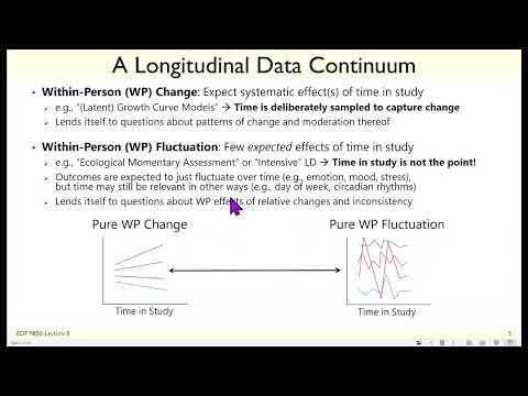
Within-person change designs space measurements to capture a sustained process, such as treatment response over weeks or human development measured over years.
Growth-curve models examine whether trajectories are linear or nonlinear and whether person-level characteristics explain differences in change.
Ecological momentary assessment and daily-diary designs sample frequent fluctuations in states such as mood, stress, affect, and social support.
Fluctuation studies can also examine person-to-person differences in within-person residual variance, such as emotional instability or inconsistent medication adherence.

16:16 Spring Break Drinking and Measurement-Burst Examples

A Penn State student study tracked college students’ weekly intended alcohol consumption across three cohorts; aligning time to spring break revealed a shared event-related increase obscured by cohort start dates.
A binary spring-break contrast was more interpretable than a quadratic semester trend, and its random slope captured how much each student expected their drinking to change.
In a measurement-burst study, older adults completed six assessments over two weeks, with the burst repeated every six months; negative affect rose across bursts but declined within some bursts.
The examples show that designs intended to study fluctuation may also contain systematic time effects, including changes associated with a salient event or repeated interviewer visits.

22:42 Time Metrics, Accelerated Designs, and Balanced Schedules

Choose a time metric that matches the mechanism: time in study, age, grade, or time since a disease diagnosis can answer different questions.
Fluctuation studies may need time of day or day of week rather than a linear time-in-study trend; intensive designs can require separate time scales for hours and days.
Balanced designs share the same possible measurement occasions across people, as in pretest, posttest, and follow-up schedules; missed observations do not change the schedule itself.
Unbalanced designs have different occasion times across people, as when participants enter at different ages, and offer fewer modeling options than balanced designs.

26:44 Why Repeated Outcomes Need Dependence Models

Ignoring within-person correlation can produce incorrect standard errors, p-values, and—in models with time-varying predictors—biased or “smooshed” effects.
Person ID fixed effects give each person a separate intercept; person-by-time interactions can give each a separate trajectory, but this approach cannot explain differences using time-invariant predictors.
Fixed effects can be useful with very few people or when the analysis targets individual-specific conclusions, including aggregated N-of-1 randomized trials.
Hoffman outlines three ways to model dependence: person fixed effects, multivariate outcome covariance structures, and multilevel random effects.

30:41 Repeated-Measures ANOVA and Alternative Covariance Structures

The repeated-measures ANOVA univariate approach assumes compound symmetry: equal residual variances and equal correlations across occasions, equivalent to a random-intercept model.
An unstructured multivariate model estimates a separate variance for each occasion and correlation for every pair, but becomes unwieldy with many occasions or few people.
Ordinary least squares excludes people missing any outcome; likelihood-based estimation such as REML or ML can retain incomplete cases under the model’s assumptions.
Compound symmetry with heterogeneous variances permits variances to change while correlations remain equal; autoregressive and moving-average structures are other options.

34:35 Random Effects and AR(1) Residual Correlation

A random intercept creates constant person-level dependence, while random slopes allow the covariance pattern to vary across occasions.
Random-effects models can handle continuous, categorical, and count outcomes as well as balanced or unbalanced schedules and incomplete observations.
An AR(1) residual structure models remaining correlation after random effects: adjacent occasions correlate by R, two lags by R², and three lags by R³.
Hoffman notes that continuous-time autoregressive residual options are available in R and SAS; the R package lme4 does not provide general residual covariance structures beyond its standard setup.

37:32 Testing Fixed and Random Effects of Time

A non-flat average trajectory indicates a fixed effect of time; differences in individual trajectories indicate a random slope.
If everyone changes by the same amount, a fixed time slope with a random intercept produces parallel trajectories and can preserve compound symmetry.
If individuals change in different directions or at different rates, a random slope is needed and the variance can change over time.
Time should be coded on a meaningful scale: occasions at weeks 0, 4, and 8 should not automatically be coded 1, 2, and 3 if the coefficient is meant to represent change per week.

40:10 Empty Means Models, ICC, and Covariance Matrices

An empty random-intercept model separates between-person variance in average outcomes from within-person residual variance across occasions.
The longitudinal ICC is the between-person random-intercept variance divided by total variance; it represents the expected correlation between occasions from the same person.
The random intercept accounts for dependence but does not explain why people have different means; explanatory predictors are needed for that.
In Hoffman’s matrix notation, G holds level-two random-effect variances and covariances, R holds level-one residual variances and covariances, and V combines them into the marginal covariance pattern.

47:45 Random Linear Slopes: Person-Specific Change and Variance

Adding a fixed linear time slope estimates the average change; adding a random time slope lets each person deviate from that rate.
With a random intercept and slope, the intercept is conditional on time zero, and the model estimates the covariance between a person’s starting level and rate of change.
The random slope makes trajectories nonparallel and induces time-dependent variance and covariance; variance can increase as people’s trajectories spread apart.
The model’s G matrix contains intercept variance, slope variance, and their covariance, while the standard version assumes constant, independent level-one residuals.

57:39 A Longitudinal Modeling Workflow and What Comes Next

Begin with empty models for every repeated variable to assess between-person variation; most time-varying predictors have both within-person and between-person components.
Plot observed means when data are complete; with attrition or other missingness, fit a categorical-time model to estimate occasion means using likelihood-based estimation.
Evaluate fixed and random time effects, then assess whether residual correlation in the level-one R matrix is needed, especially in intensive fluctuation designs.
Person-mean centering is usually appropriate for time-varying predictors to separate within-person effects from between-person averages; the next lecture section applies this to stress and disease severity, quadratic change, and piecewise models.

Summary, takeaways, and chapters were generated by AI from the video's transcript and may contain errors. The video belongs to its creator, Lesa Hoffman.