Dynamics (MIT 16.07) - Lecture 9: Spinning Stability

Overview

Torque-free rigid-body motion is described geometrically as the intersection of a fixed angular-momentum sphere and kinetic-energy ellipsoids, explaining why spins about the minor and major inertia axes are stable while the intermediate-axis spin is unstable. The lecture derives this result with local linear stability analysis of Euler’s equations, then connects energy dissipation—from fluid slosh, flexible-mode damping, or eddy currents—to the eventual flat spin about the major axis.

Key takeaways

For a torque-free rigid body with J₁ < J₂ < J₃, fixed angular momentum makes the major-axis spin the energy minimum and the minor-axis spin the energy maximum; both are stable, while the intermediate-axis spin is unstable.
The T-wrench flip follows a separatrix connecting the two unstable intermediate-axis equilibria; smaller initial perturbations delay the flip because the motion remains near the unstable spin longer.
At fixed angular-momentum magnitude, kinetic energy is T = ½HᵀJ⁻¹H, so spinning about the smallest moment of inertia requires the most energy and spinning about the largest requires the least.
Linear stability analysis uses the Jacobian eigenvalues: negative real parts imply local asymptotic stability, a positive real part implies instability, and zero real parts require caution for nonlinear systems.
Internal dissipation can move a body across conservative trajectory boundaries and drive it toward the major-axis flat spin; examples include fluid slosh, flexible-mode damping, and eddy-current losses.
Minor- and major-axis perturbations yield purely imaginary eigenvalues in the linearized equations, corresponding to bounded oscillatory wobble rather than exponential growth.

Chapters

0:00 The T-Wrench and the Intermediate-Axis Flip

The opening T-wrench demonstration shows a body nearly spinning about its intermediate principal axis before it flips.
In torque-free motion, trajectories lie at the intersection of a fixed angular-momentum sphere and a kinetic-energy ellipsoid.
A tiny perturbation from the intermediate-axis spin grows exponentially, although a smaller perturbation delays the visible flip.

3:00 From Euler’s Equation to Spin Stability

The lecture revisits Euler’s equation, angular momentum, and the principal-axis equilibria established in the previous class.
It sets up a local stability analysis before moving on to attitude representations, which describe orientation rather than angular velocity.

5:30 Equilibrium Spins Align with Inertia Eigenvectors

An equilibrium point satisfies ẋ = f(x) = 0; for a spinning body, equilibrium means angular velocity remains constant even as the body rotates.
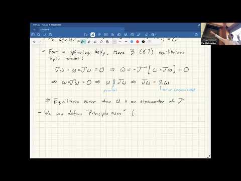
Euler’s equation gives ω × Jω = 0, so equilibrium requires Jω = λω: the spin direction must be an eigenvector of the inertia matrix.
The six signed equilibrium directions correspond to the positive and negative directions of the three principal axes.

11:00 Principal Axes and the Ordered Inertia Values

The principal-axis frame uses inertia eigenvectors as its basis, making the inertia matrix diagonal.
The moments are ordered J₁ < J₂ < J₃: the minor, intermediate, and major axes of inertia, respectively.
The inertia matrix and its inverse share eigenvectors, while their eigenvalues are reciprocals.

14:30 Kinetic Energy at Fixed Angular Momentum

Kinetic energy can be written as T = ½ωᵀJω or, using H = Jω, as T = ½HᵀJ⁻¹H.
For the same angular-momentum magnitude, rotation about the minor axis has the greatest kinetic energy because J₁ is smallest.
Rotation about the major axis has the least kinetic energy because J₃ is largest; the intermediate-axis energy lies between them.

20:00 Energy Ellipsoids Touch the Momentum Sphere at Equilibria

The angular-momentum sphere stays fixed in torque-free motion, while the energy ellipsoid changes size with kinetic energy.
At the major-axis energy minimum and minor-axis energy maximum, the ellipsoid just touches the sphere at the corresponding equilibrium directions.
Reducing the energy from an extremum produces an intersection curve that represents a non-equilibrium trajectory.

24:00 Mutation Orbits and the Separatrix

Small perturbations around the minor- and major-axis spins produce bounded periodic wobbling, called mutation in the lecture.
The intermediate-axis equilibria are unstable, and a separatrix divides the surrounding regions of motion.
The separatrix connects the two unstable intermediate-axis equilibria, creating the heteroclinic connection associated with the T-wrench flip.

31:00 How Dissipation Moves a Body Between Spin Regimes

With energy conserved, a torque-free trajectory cannot cross the separatrix; energy dissipation shrinks the energy ellipsoid and can carry the motion across it.
Because the major-axis spin is the global energy minimum at fixed angular momentum, dissipation ultimately favors that flat spin.
Fluid slosh in fuel tanks and damping in flexible spacecraft structures are practical sources of internal energy loss.

35:00 ISS Demonstrations and Asteroid Spin-Down

Astronaut Don Pettit’s ISS demonstrations show stable minor-axis rotation and flipping about the intermediate axis.
A solid cylinder can maintain its spin for a long time, while a bottle or raw egg dissipates energy through moving internal fluid and settles toward a flat spin.
Asteroids can also reach flat spin over long periods; metallic objects may dissipate energy through eddy currents in magnetic fields, a mechanism also used in roller-coaster brakes.

39:00 Euler’s Equations in Principal-Axis Coordinates

Diagonalizing inertia reduces Euler’s equation to three coupled component equations for ω₁, ω₂, and ω₃.
The cross-product terms vanish when rotation is confined to one principal axis, making each principal-axis spin an equilibrium.
An external torque adds torque components to the equations and breaks the conserved angular-momentum and energy picture used for torque-free motion.

42:00 One-Dimensional Stability from the Dynamics Slope

For a scalar system ẋ = f(x), equilibria occur at roots of f(x); the sign of f around each root shows whether nearby motion returns or moves away.
A negative derivative f′(x*) indicates local stability, while a positive derivative indicates instability.
If f′(x*) = 0, linearization is inconclusive: cubic examples can have zero slope at equilibrium yet be stable or unstable depending on higher-order terms.

52:00 Jacobian Eigenvalues Generalize the Stability Test

For ẋ = f(x) in n dimensions, the derivative at equilibrium is the square Jacobian A = ∂f/∂x.
Eigenvalues with strictly negative real parts imply local asymptotic stability; any eigenvalue with a positive real part implies instability.
Zero real parts make the linear test inconclusive for a nonlinear system, so further nonlinear analysis may be required; in a controlled system, the input Jacobian is conventionally called B.

1:01:00 Minor-Axis Spin Linearization Produces Oscillations

Linearizing about ω₁ = ωₖₙ drops the second-order perturbation term in the ω₁ equation, leaving the nominal spin constant to first order.
The perturbation equations for ω₂ and ω₃ form a coupled 2 × 2 linear system with coefficients of opposite signs.
Its eigenvalues are purely imaginary, predicting bounded oscillatory motion; this supports stability and corresponds to the wobble seen in the demonstrations.

1:10:00 Intermediate-Axis Instability and Major-Axis Stability

Linearization about the intermediate axis gives two negative coefficients whose product is positive, producing one positive and one negative real eigenvalue.
The unstable eigenvalue explains exponential departure from the intermediate-axis equilibrium, while the stable direction describes how trajectories approach it along the separatrix.
The major-axis linearization gives purely imaginary eigenvalues like the minor-axis case; without dissipation both axes are stable, but with dissipation the major-axis flat spin is the surviving energy minimum.

Summary, takeaways, and chapters were generated by AI from the video's transcript and may contain errors. The video belongs to its creator, MIT Robotic Exploration Lab.