Dynamics, Lectures 3 & 4: Oxford Mathematics 1st Year Student Lecture

Overview

This lecture from Oxford Mathematics explores fundamental forces and energy concepts in classical mechanics. It details Hooke's Law for springs, deriving simple harmonic motion, and introduces the Lorentz force for charged particles in electromagnetic fields, illustrating cyclotron motion. The lecture then transitions to energy, defining kinetic and potential energy, conservative forces, and the principle of energy conservation, demonstrating its application with examples like a falling ball and a spring-mass system, and introducing the concept of energy landscapes for analyzing motion.

Key takeaways

Hooke's Law (F = -KΔX) describes ideal spring behavior, leading to simple harmonic motion (X(t) = D cos(ωt) with ω = √(K/M)).
The Lorentz force (F = Q(E + V × B)) governs charged particle motion in electromagnetic fields, resulting in helical trajectories (cyclotron motion) in constant magnetic fields.
For conservative forces, total energy (Kinetic + Potential) is conserved (E = T + V = constant), allowing analysis of motion via energy landscapes.
Potential energy V(X) defines an 'energy landscape'; motion is analogous to a ball rolling on this landscape, with acceleration determined by the slope (-V'(X)).
The convergence of the time integral ∫ dX / √(E - V(X)) determines if a system reaches a state in finite or infinite time.
Equilibrium points (where F=0, V'(X)=0) are classified as stable (particle returns when nudged) or unstable (particle moves away when nudged) based on the local shape of the potential energy landscape.

Chapters

0:00 Review of Dry Friction and Introduction to Spring Force

Recap of dry friction, emphasizing the inequality for friction force magnitude.
Introduction to the spring force as a key force in dynamics.
Mention of Hooke's Law as the governing principle for spring forces.

2:12 Hooke's Law and Spring Force Derivation

Description of a spring attached to a mass with rest length L.
Explanation of Hooke's Law based on Robert Hooke's 17th-century experiments.
Derivation of the spring force vector: F = -K(X - L)êx, where K is the spring constant.

9:57 Newton's Second Law for a Spring-Mass System

Application of Newton's second law: M Ẍ = F.
Scalar equation for 1D motion: M Ẍ = -K(X - L).
Initial conditions: X(0) = L + D, Ẋ(0) = 0.

15:30 Simplifying the Spring-Mass Equation with Displacement Variable

Definition of a new variable Y(t) = X(t) - L to represent displacement from rest length.
Transformed differential equation: M Ÿ = -K Y.
New initial conditions: Y(0) = D, Ÿ(0) = 0.

17:38 Solution of the Simple Harmonic Motion Equation

Identification of the equation as simple harmonic motion.
General solution: Y(t) = A cos(ωt) + B sin(ωt).
Definition of angular frequency: ω = √(K/M).

19:06 Units of Angular Frequency and Initial Conditions

Units of ω are 1/time (frequency).
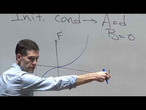
Applying initial conditions Y(0)=D, Ÿ(0)=0 yields A=D, B=0.
Specific solution: Y(t) = D cos(ωt).

22:04 Limitations of Hooke's Law and Real Spring Behavior

Hooke's Law is an empirical observation valid for small displacements.
Real springs exhibit non-linear behavior at large extensions or compressions.
Real springs can fracture or reach limits of compression.

25:13 Introducing Damping Force to the Spring System

Addition of a linear damping force: F_D = -B Ẋ.
Modified differential equation: M Ÿ + B Ÿ + K Y = 0.
The damping term causes oscillations to die out.

27:21 Scenarios of Damped Oscillations

Analysis based on the discriminant B² - 4MK.
Overdamping (B² - 4MK > 0): purely exponential decay, oscillations die out quickly.
Underdamping (B² - 4MK < 0): damped oscillations with a decaying amplitude (e^(-Bt/2M) cos(ω't)).

30:24 Overview of Forces in Dynamics

Recap of forces: gravity, springs, damping.
Mention of electromagnetic forces as another example.
Note that damping forces often make mathematical analysis more complex.

30:44 Introduction to the Lorentz Force

Force on a charged particle (Q) in electric (E) and magnetic (B) fields.
Lorentz force equation: F = Q(E + V × B).
QE term is force along electric field lines; QV×B is orthogonal to V and B.

35:48 Trajectory of a Particle in a Constant Magnetic Field

Simplification: constant B, no E field, particle starts at origin.
Without loss of generality, align B with Z-axis (B = B êz).
Initial velocity can be rotated to have only X and Z components: V(0) = V₁ êx + V₃ êz.

42:11 Integrating the Lorentz Force Equation

First integration of Newton's second law (M R̈ = Q V × B): M Ṙ = Q R × B + C.
Constant vector C determined by initial velocity: C = M V(0).
Decomposition into components: M Ẋ = Q(Y B - V₃), M Ÿ = Q(-X B + V₂), M Ż = Q(X B - V₁).

45:12 Coupled Motion in X and Y, Decoupled Motion in Z

Z-component equation: M Ż = 0 (since V₂=0), leading to Z(t) = V₃t.
Coupled equations for X and Y: Ẋ = ωY + V₁, Ÿ = -ωX, where ω = QB/M.
The motion in X and Y is coupled, while Z moves at a constant velocity.

47:14 Solving for X and Y Components of Motion

Differentiating Ẋ to get Ẍ = ωŸ = -ω²X, resulting in simple harmonic motion for X.
Solution for X(t): X(t) = (V₁/ω) sin(ωt) (using X(0)=0, Ẋ(0)=V₁).
Solution for Y(t): Y(t) = (V₁/ω) cos(ωt) - 1 (derived from Ÿ = -ωX).

50:00 Cyclotron Motion and Particle Accelerators

The trajectory is a helix: circular motion in the XY plane and constant velocity motion in Z.
ω = QB/M is the cyclotron frequency.
Adding an electric field can lead to accelerating motion, forming the basis of particle accelerators.

53:24 Introduction to Energy Concepts: Kinetic and Potential Energy

Transition to energy formulation for understanding motion.
Kinetic Energy (T): T = ½ m Ẋ² (energy of motion).
Potential Energy (V): Defined for conservative forces, V(X) = -∫ F(s) ds.

1:00:04 Properties of Potential Energy and Conservative Forces

V'(X) = -F(X).
If F=0, then V=constant (no potential energy).
Potential energy definition requires forces to be functions of position only (conservative forces), excluding drag or magnetic forces.

1:03:54 Conservative Forces and Energy Conservation

Forces for which potential energy can be defined are called conservative.
Examples of non-conservative forces: drag, friction.
For conservative forces, total energy (T + V) is conserved.

1:09:11 Work Done by a Force and Energy Change

Work (W) done by force F moving a particle from x₁ to x₂: W = ∫ F(s) ds from x₁ to x₂.
Work-Energy Theorem: W = V(x₁) - V(x₂) = -ΔV.
Work done by a conservative force equals the negative change in potential energy.

1:17:20 Conservation of Energy Principle

Total energy E = T + V is constant for conservative systems.
Deduction from Newton's second law: d/dt (½ m Ẋ² + V(X)) = 0.
Energy is interconverted between kinetic and potential forms.

1:30:13 Example: Projectile Motion Under Gravity

Ball thrown upwards from X=0 with velocity V₀.
Force F = -mg, Potential Energy V(X) = mgX.
Total energy E = ½ m V₀² (at t=0, V(0)=0).
Maximum height reached when kinetic energy is zero, so E = mg X_max.

1:36:41 Example: Spring-Mass System Energy Analysis

Spring force F = -K(X - L), Potential Energy V(X) = ½ K (X - L)².
Total energy E = ½ m Ẋ² + ½ K (X - L)².
At maximum displacement (X=L±D), Ẋ=0, so E = ½ K D².
At equilibrium (X=L), V=0, so E = ½ m Ẋ_max².

Summary, takeaways, and chapters were generated by AI from the video's transcript and may contain errors. The video belongs to its creator, Oxford Mathematics.