CMU Introduction To Deep Learning 11-785, Fall 2026: Lecture 9

Overview

The lecture derives convolutional neural networks from the goal of recognizing patterns regardless of where they appear: a shared-parameter MLP scans an input, and its computation can be reorganized into layers of local filters. Distributing pattern recognition across layers creates hierarchical features, reduces parameters and repeated computation through weight sharing and reuse, and leads to CNN concepts including feature maps, receptive fields, stride, flattening, and pooling.

Key takeaways

A shared-parameter detector achieves shift-invariant recognition by applying the same local network at every input position, then aggregating local detections with a max-like operation.
When multiple network connections represent copies of one shared weight, backpropagation must sum the gradients from every copy; the update is not based on averaging them.
CNN computation can be reordered so each layer scans the previous layer’s feature maps, preserving the result of scanning the full MLP while exposing reusable intermediate activations.
Distributing a width-eight detector across smaller receptive fields lets lower layers detect local features and higher layers combine them, reducing parameter counts compared with an undivided network.
Overlapping convolution windows reuse already computed features, reducing the additional computation needed as the scan advances.
Pooling selects the strongest activation within a local region, providing tolerance to small spatial shifts in features such as flower petals.

Chapters

0:00 Lecture Setup and Convolutional-Network Homework

The class is beginning a unit on convolutional neural networks, which will soon connect to homework.
The opening includes attendance checks using randomly called Pokémon names and a reminder to focus on the lecture.

5:22 Why Ordinary MLPs Miss Shifted Patterns

An MLP trained to detect “hello” at one point in a one-second spectrogram may miss the same word at another time.
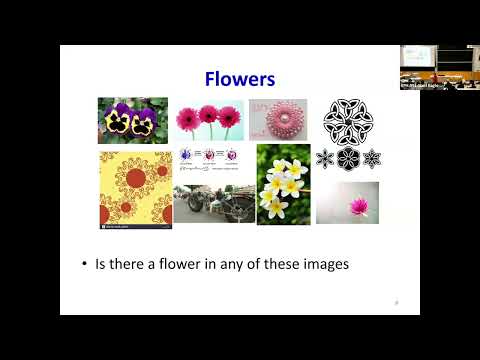
In images, a flower moved from the top-left corner changes which input dimensions activate, so a location-specific MLP may fail.
Shift invariance means recognizing a pattern’s presence regardless of its position; conventional fully connected MLPs are location-sensitive.

9:51 Sliding-Window Detection and Max Aggregation

A small MLP can inspect a window the size of a target, such as the word “welcome,” while sliding across the input.
The window-level outputs are combined into a recording-level decision using a maximum or an approximation such as softmax.
The maximum implements an “at least one location” rule: one strong detection can make the whole recording positive.

13:55 Shared Subnetworks Turn Scanning into One Large MLP

Scanning a picture with a flower detector is equivalent to applying the same small MLP at every image location.
The scanned windows form one large network whose repeated subnetworks have identical parameters.
Parameter sharing builds location independence into the architecture instead of requiring training examples at every possible location.

20:12 Training Shared Weights Requires Summing Gradients

Training examples need only image- or recording-level labels; they do not need annotations marking the target’s exact position.
When several network edges are copies of one shared parameter, the gradient for that parameter is the sum of the gradients through all its copies.
The copies can receive different local gradients because they process different input values, but their contributions update the same shared weight.

29:06 Reordering Computation Across Positions and Layers

Computing the full MLP at every input position can be reordered: each layer processes all positions before the next layer runs.
The final output remains unchanged because the computations over positions and layers are independent outer loops around the same neuron-level operations.
For images, first-layer neurons can produce maps over the input, and later layers can read the relevant map locations.

36:38 Feature Maps Preserve the Original Scanning Results

Each first-layer neuron produces a map showing where its learned pattern responds across the input.
To classify a particular region, later-layer outputs are gathered from the corresponding positions in the preceding layer’s maps.
Processing the maps layer by layer yields the same location-specific result as passing each full window through the complete MLP.

44:24 Distributing a Flower Detector Across Layers

Instead of asking first-layer neurons to detect an entire flower-sized window, they can detect smaller features such as petals or other local structures.
Second-layer neurons inspect windows of first-layer maps, combining local responses into larger patterns.
This distributes responsibility across layers while retaining a final decision for each image location.

53:27 Weight Sharing in Multi-Layer Pattern Recognition

Even when recognition is distributed across layers, the network still behaves as an MLP scanning the input; the organization of shared parameters changes.
The lecture’s example has three first-layer feature types, each applied across locations, so a higher-layer window can use 27 activations derived from just three shared parameter sets.
Adding layers lets the network build larger receptive regions from smaller local features rather than requiring one first-layer detector for the whole object.

58:07 Convolution, Filters, and Time-Delay Networks

Scanning a window over the previous layer’s outputs is implemented as a dot product with shared weights, called a filter.
The scanning operation is commonly called convolution, although the lecture notes that the usual neural-network operation is technically cross-correlation.
Stacked feature maps and filter weights form tensor-shaped inputs and parameters; the one-dimensional version is also known historically as a time-delay neural network.

1:02:59 Why CNNs Distribute Pattern Recognition

Distributed scanning requires map locations to retain their spatial arrangement because later layers inspect adjacent windows.
Lower layers can represent localized features and higher layers can compose them into more complex patterns.
The architectural goal is a hierarchical representation that uses fewer parameters and computations than a large, undivided detector.

1:06:44 Hierarchical Features Improve Model Efficiency

Neural networks can construct complex patterns from simple ones across layers, such as combining petal-like features into flower-like structures.
Distributing a complex decision across layers can use a more compact network than representing it with a single hidden layer.
The lecture connects this hierarchical structure to improved data and parameter efficiency and potentially better generalization.

1:08:35 Counting CNN Computations with an Eight-Vector Window

For a window of eight vectors, each of dimension D, a non-distributed first layer with 4N1 neurons performs 8D × 4N1 multiply-accumulate computations.
A distributed version can use width-two first-layer windows, with later layers combining their outputs to cover the same effective width of eight.
Smaller local operations reduce the work required at each position, and later processing can reuse feature values already computed for overlapping regions.

1:14:58 Parameter Sharing and Reuse Reduce Total Work

The lecture compares networks with the same overall neuron layout: in the distributed version, groups of first-layer neurons share weights.
For a width-eight example split across layers, the distributed network has far fewer unique parameters than an undivided network with the same number of neurons.
Overlapping windows allow computations to be reused as the scan advances, so each step adds only a small amount of new work.

1:20:54 CNN Design Trade-Offs and Core Terminology

Weight sharing reduces the number of distinct parameters, but it does not remove the need to represent the scanning activations in memory.
A filter’s receptive field is the input region that influences its neuron; receptive fields generally grow in deeper layers.
Stride greater than one shrinks feature maps, and converting map outputs into a vector is called flattening.

1:24:26 Pooling Adds Tolerance to Small Shifts

A flower remains a flower when a petal shifts slightly, so recognition should tolerate small changes in the positions of component features.
Pooling examines a local window and selects its largest activation, allowing limited jitter in lower-level patterns.
The lecture’s CNN structure combines learned filters, hierarchical feature maps, optional stride, flattening, and pooling.

Summary, takeaways, and chapters were generated by AI from the video's transcript and may contain errors. The video belongs to its creator, Carnegie Mellon University Deep Learning.