CMU Introduction To Deep Learning 11-785, Fall 2026: Lecture 8

Overview

Lecture 8 closes the neural-network training unit by connecting loss choice and gradient descent to generalization techniques: cross-entropy for classification, batch normalization for mini-batch variation, and regularization, depth, and dropout for overfitting. It derives how batch normalization changes backpropagation, explains dropout as an efficient approximation to averaging an exponential family of subnetworks, and ends with practical training heuristics and a validation-based workflow.

Key takeaways

For classification, cross-entropy/KL paired with sigmoid or softmax produces a well-behaved loss in logit space and a simple output gradient of prediction minus target; squared error can become nonconvex after the activation.
Batch normalization computes per-neuron mini-batch statistics, normalizes activations, then restores flexibility with learnable γ and β; its batch-dependent statistics make gradients couple examples.
Batch normalization relies on representative, diverse mini-batches: if all examples are identical, the lecture’s gradient analysis shows that backpropagation can be blocked.
L2 regularization penalizes large weights and yields weight decay, while network depth can constrain the learned function’s complexity—though excessive depth under a fixed parameter budget can make layers too narrow.
Dropout samples subnetworks by independently masking neurons during training; its 2ⁿ possible networks share weights, and inference approximates their ensemble with keep-probability scaling.
Validation-based early stopping, input augmentation, gradient clipping, normalization, and careful initialization complement the choice of optimizer and architecture in a practical training pipeline.

Chapters

0:00 Class Setup and Attendance

The class handles attendance and arranges Zoom chat monitoring before the lecture begins.
The opening minutes include classroom logistics rather than technical material.

6:00 Training Recap and the Shift to Generalization

The course has covered neural-network basics and several weeks of training methods; convolutional neural networks begin next week.
Training minimizes average divergence over samples as an approximation to expected error, using gradient descent.
Batch updates process the full training set, while stochastic and mini-batch updates are faster but noisier; trend-based methods smooth their fluctuations.

9:00 Why the Shape of a Divergence Function Matters

A useful divergence is nonnegative and reaches zero when the network output matches the target.
Gradient descent behaves poorly on a function with small slopes far from the optimum and steep slopes near it.
A desirable loss gives large corrective gradients far from the answer and smaller steps near the minimum.

12:00 L2 Versus KL Loss for Classification Logits

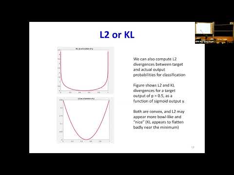
For a binary example with target probability 0.5, L2 loss is quadratic in the predicted probability, while KL loss becomes unbounded for confidently incorrect predictions.
The output probability is produced by applying a logistic or softmax activation to a pre-activation logit.
Although L2 looks well behaved as a function of probability, its composition with the logistic activation is nonconvex in the logit; cross-entropy/KL gives a convex objective in that setting.

16:00 Output-Layer Gradients and Checking Their Sign

For regression with identity activation and classification with sigmoid/softmax plus cross-entropy, the logit gradient simplifies to prediction minus target, y − d.
The same prediction-minus-target form arises for squared error with a linear regression output.
A directional check confirms the sign: when y exceeds d, increasing y raises squared error, so the derivative must be positive.

21:00 Mini-Batch Variation and Internal Covariate Shift

Mini-batches may differ substantially from the full dataset’s distribution, so an update can pull the model toward a batch-specific solution.
Nonlinear layers can send initially similar batches to different regions of representation space.
Batch normalization addresses this variation by centering and scaling each neuron’s mini-batch activations before learning a shift and scale.

26:00 Batch Normalization: Normalize, Then Learn Scale and Shift

For each neuron and mini-batch, compute the mean and variance, then normalize each affine output z as u = (z − μ) / √(σ² + ε).
Learnable parameters γ and β produce the adjusted activation input ẑ = γu + β.
The small ε term prevents division by zero; β restores a learnable offset, making the preceding affine bias unnecessary.

30:00 Why Batch Normalization Couples Examples in Backpropagation

Without batch normalization, each example’s loss can be differentiated independently before averaging gradients across the mini-batch.
With batch normalization, each example’s normalized value depends on the batch mean and variance, so its output and loss depend on other examples.
The gradients for γ, β, and u follow directly from ẑ = γu + β; the more involved part is propagating gradients back through shared batch statistics.

36:00 Deriving Batch-Norm Gradients Through the Computation Graph

For any zᵢ, the gradient sums contributions from every uⱼ because zᵢ affects the batch mean, variance, and all normalized outputs.
The derivation tracks direct paths through zᵢ, indirect paths through μ, and paths through σ² using the chain rule.
Computing one neuron at a time across the mini-batch keeps the dependency graph manageable; each neuron has its own batch statistics.

45:00 Batch Diversity and Inference-Time Statistics

If every example in a mini-batch is identical, the lecture’s batch-normalization gradient derivation yields zero gradients, blocking useful backpropagation.
Randomized, diverse mini-batches are therefore important for batch normalization to represent the data distribution.
At inference, running estimates of the mean and variance are used because single-example predictions do not provide a mini-batch to compute them from.

53:00 Under-Specified Data and the Need for Smooth Functions

A network can fit training samples while behaving implausibly between them because the training loss constrains only observed points.
The lecture’s binary-classification example contrasts a jagged boundary that fits samples with a smoother boundary preferred for generalization.
Large sigmoid weights can make activations nearly step-shaped, allowing sharp changes between data points.

59:00 L2 Weight Regularization and Weight Decay

Adding λ‖w‖² to the data loss discourages large weights while still minimizing training divergence.
Differentiating the penalty adds a term proportional to λw to the gradient.
The resulting update includes multiplicative shrinkage of weights, the operation known as weight decay.

1:05:00 Depth as a Constraint on Decision-Boundary Complexity

The lecture presents depth as a way to compose smoother transformations, potentially producing less jagged functions than unconstrained shallow networks.
In examples with 1,000 training samples and roughly 660 neurons, deeper arrangements better approximate the illustrated bolt- and bear-shaped decision boundaries.
Depth is not unlimited: with a fixed neuron budget, layers can become too narrow and hurt performance.

1:09:00 Dropout as Stochastic Bagging

Bagging trains multiple models on different data samples and combines their predictions; dropout approximates this idea within one network.
During training, each neuron is independently kept with probability α or switched off with probability 1 − α for a particular example.
A network with n neurons has up to 2ⁿ possible dropout subnetworks, which share weights rather than requiring separate training runs.

1:13:00 Dropout Masks, Inference Scaling, and Batch-Norm Compatibility

A Bernoulli mask zeros selected neuron outputs during the forward pass and is reused during backpropagation for that training example.
At inference, the lecture approximates averaging subnetworks by using all neurons and scaling each output by the keep probability α.
Dropout can make activation variance inconsistent with batch-normalization statistics, so combining the methods is often ineffective in the settings discussed.

1:19:00 Training Heuristics: Clipping, Early Stopping, and Augmentation

Gradient clipping limits extreme derivatives that could destabilize optimization.
Early stopping monitors a held-out validation set and halts training when validation error begins to rise.
Data augmentation perturbs inputs while preserving their labels, encouraging locally smooth predictions; input standardization and careful initialization are also recommended.

1:24:00 End-to-End Neural-Network Training Workflow

Choose training data, a network architecture, a suitable divergence, regularization, and optimization methods such as Adam.
Tune hyperparameters with a grid search on held-out data and evaluate periodically on validation data for early stopping.
The lecture closes the training unit by emphasizing hands-on experiments alongside gradient-based optimization, regularization, and convergence heuristics.

Summary, takeaways, and chapters were generated by AI from the video's transcript and may contain errors. The video belongs to its creator, Carnegie Mellon University Deep Learning.