CMU Introduction To Deep Learning 11-785, Fall 2026: Lecture 7

Overview

The lecture develops mini-batch gradient descent as a practical middle ground between full-batch updates and single-example SGD, explaining how random shuffling, learning-rate schedules, and batch size affect convergence and variance. It then connects noisy incremental updates to trend-based optimizers—momentum, Nesterov momentum, RMSProp, and Adam—and explains how each uses gradient history or squared gradients to stabilize training.

Key takeaways

Full-batch gradient descent processes every training example before updating, whereas single-example SGD makes an immediate update after each sample and performs T updates per epoch for T examples.
Randomly permuting examples within each epoch reduces order-driven oscillation that can occur when consecutive groups produce opposing gradients.
A learning-rate schedule must balance two requirements: the sum of step sizes diverges so training can travel far enough, while the sum of squared step sizes converges to limit persistent noise.
A mini-batch of b independent examples gives an unbiased objective estimate whose variance scales as 1/b, trading lower gradient noise against fewer updates per epoch and greater per-update computation.
Momentum smooths gradients over time, RMSProp scales updates using running averages of squared gradients per parameter, and Adam combines both mechanisms with bias correction.
Even correctly computed SGD gradients can vary sharply from sample to sample; this higher variance can speed early progress while making convergence noisier and final solutions less reliable than full-batch training.

Chapters

0:00 Classroom Setup and Pokémon Attendance Polls

The class begins with attendance logistics, name tags, and Pokémon-themed polling.
At about 5:00, the lecture turns to neural-network training; convolutional networks are announced for the following week.

5:00 Empirical Risk Minimization and Gradient Descent Recap

A neural network with weights W represents a function that approximates an unknown input-output relationship.
Training data provide sampled input-target pairs, so the average divergence on those examples serves as a proxy for error across the full data distribution.
Gradient descent updates W in the direction that reduces loss, using backpropagation to calculate derivatives.

12:00 Why Full-Batch Updates Become a Bottleneck

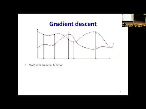
A batch update averages divergence and gradients across every training example before changing any parameter.
That approach can require processing billions or trillions of examples for a single update, making it impractical for very large datasets.
The putty-shaping analogy illustrates the alternative: make a sequence of smaller local corrections rather than waiting to adjust everything at once.

18:00 Incremental Updates and the Meaning of an Epoch

Incremental training computes one example's divergence and gradient, then updates network parameters immediately.
An epoch is one complete pass through the training set; with T examples, single-example SGD makes T updates per epoch.
Training can make multiple epochs, applying repeated small corrections to improve the model.

21:00 Shuffle Examples to Prevent Oscillating Updates

Processing examples in a fixed order can create cyclic behavior: one group may push a function down, while the next pushes it back up.
Randomly permuting the training examples within every epoch mixes those competing corrections.
This randomized, incremental procedure is stochastic gradient descent (SGD).

24:00 Why SGD Can Make Progress with Individual Examples

Each training example can produce a different gradient, but averaging their directions gives the full-data correction.
If examples are identical, each gradient points the same way, so successive incremental updates can accumulate more movement than a single batch update.
When examples are broadly representative and step sizes are controlled, incremental updates can approximate the direction indicated by the whole dataset.

29:00 Decaying Learning Rates and the Principal-Axis Example

In an incremental principal-axis example, each new point can pull the estimated axis toward itself; large steps make the estimate swing between points.
Shrinking the learning rate lets later examples influence the estimate without erasing evidence from earlier examples.
The lecture derives two conditions for step sizes ηₖ: their sum must diverge, while the sum of their squares must converge.
A schedule proportional to 1/k satisfies these conditions; practical schedules may instead hold the rate steady and reduce it when progress plateaus.

39:00 SGD Convergence Speed, Variance, and Limitations

An illustrated comparison shows SGD reaching a solution faster than batch updates but with higher run-to-run variance and potentially worse final error.
For a neural network, the bound on gradient-driven movement depends not only on activation slopes but also on weight matrices; their largest singular values can amplify changes.
Convergence requires learning rates to shrink enough to limit persistent oscillation while retaining an infinite total step length.

48:00 Why Training Loss Estimates the Full-Data Objective

The actual objective is expected divergence over the data distribution, weighted by how likely each input is to occur.
For randomly sampled training examples, the expected sample-average loss equals that full-distribution objective, making it an unbiased estimate.
The variance of an average over n independent, identically distributed examples scales as 1/n.

57:00 Single-Example SGD Produces Noisy Recommendations

Different random sets of six examples can recommend contradictory changes to the same function: push it up, push it down, or leave it nearly unchanged.
With SGD, each update uses one example, so its gradient estimate has much higher variance than an estimate based on many examples.
Those noisy recommendations help explain why SGD can converge quickly yet settle at a less reliable or higher-error solution.

1:00:00 Mini-Batches Balance Gradient Noise and Update Cost

Mini-batch descent averages gradients across a random subset rather than using either the full dataset or a single example.
A batch of size b remains an unbiased estimate of the full objective, with variance proportional to 1/b.
As batch size increases, the estimate becomes more reliable and approaches full-batch behavior; SGD is the special case b = 1.

1:05:00 Choosing a Mini-Batch Size in Practice

The lecture recommends using the largest mini-batch that available hardware can process without worsening overall compute time.
Larger batches reduce gradient variance but yield fewer updates per epoch and can add computation overhead.
A practical learning-rate schedule holds the rate until error plateaus, then reduces it by a fixed factor; adaptive rates are introduced as a further option.

1:10:00 Why Incremental Training Needs Trend-Based Optimizers

In SGD, the loss changes with each selected training example; in mini-batch training, it changes with each selected batch.
Consequently, gradient recommendations can swing between updates even when each gradient is correctly calculated.
Trend-based algorithms smooth those changing recommendations and are especially valuable for incremental updates.

1:12:00 Momentum and Nesterov Momentum Use Gradient History

Momentum replaces the latest gradient with a running average, smoothing direction changes across training steps.
The lecture derives a recursive update that combines the prior update with the newest gradient, avoiding the need to store every past gradient.
Nesterov momentum changes the order: it first extends the previous step, then evaluates the gradient at the resulting look-ahead position.

1:17:00 RMSProp Adapts Learning Rates by Direction

RMSProp tracks a running average of squared gradients separately for each parameter direction.
Large recurring movement in a direction signals unstable or rapidly changing gradients, so RMSProp reduces that direction's effective learning rate.
For a constant slope, the RMS magnitude cancels the gradient magnitude, leaving behavior similar to RProp's sign-based update.

1:21:00 Adam Combines Momentum with RMSProp Scaling

Adam tracks both a running average of gradients and a running average of squared gradients.
Its update uses the averaged gradient for direction and inverse root-mean-square scaling for a per-parameter step size.
Bias-correction factors compensate for initially small running averages when their decay parameters are close to one.

1:24:00 Optimizer Recap and Training Takeaways

Vanilla SGD uses the current gradient; momentum smooths gradient direction, RMSProp adapts to squared-gradient magnitudes, and Adam combines both ideas.
The lecture emphasizes shuffling, suitable learning-rate decay, and mini-batch sizing as central choices for stable and efficient training.
The class closes with recommended optimizer visualizations and a note that training-optimizer topics continue in the next lecture.

Summary, takeaways, and chapters were generated by AI from the video's transcript and may contain errors. The video belongs to its creator, Carnegie Mellon University Deep Learning.