CMU Introduction To Deep Learning 11-785, Fall 2026: Lecture 6

Overview

Lecture 6 moves from the chain-rule mechanics of backpropagation to the limits of gradient-based training: a differentiable proxy loss can favor stable solutions over perfect training-set separation, and neural-network loss landscapes can contain saddle points and local minima. Using scalar and multivariable quadratics, the class explains why one global learning rate struggles with different curvatures, then introduces learning-rate schedules, Rprop, momentum, and Nesterov’s accelerated method as ways to improve optimization.

Key takeaways

Backpropagation is a derivative-computation procedure: it propagates gradients backward through activation Jacobians and weight matrices, while a separate optimizer updates the parameters.
Optimizing a smooth proxy loss does not guarantee perfect training-set classification; its relative insensitivity to one outlier can reduce variance compared with a perceptron boundary that changes sharply.
For a scalar quadratic with curvature a, gradient descent’s one-step learning rate is 1/a, and rates above 2/a diverge; this bound becomes difficult to satisfy simultaneously when parameter directions have very different curvatures.
Hessian-based rescaling can equalize curvature in principle, but explicitly computing and inverting the Hessian is infeasible for networks with billions of parameters.
Rprop adapts each parameter’s step from consecutive gradient signs: matching signs enlarge the step, while a sign reversal triggers a rollback and smaller step.
Momentum averages successive gradient steps so consistent directions accumulate and oscillating directions cancel; Nesterov acceleration changes the order by evaluating the gradient after a momentum look-ahead step.

Chapters

0:00 Attendance and the Lecture’s Training-Algorithm Focus

The class opens with a randomized Pokémon-name attendance check, then revisits gradient descent and derivatives.
The agenda asks whether backpropagation-based training finds useful solutions and how learning-rate choices affect convergence.

5:12 Empirical Risk Minimization and Gradient Descent Recap

Neural networks are treated as universal approximators whose architecture and weights must be chosen or learned.
Empirical risk minimization minimizes average error over the observed training set rather than an unknown full data distribution.
Gradient descent updates parameters against the loss gradient; each derivative indicates how changing a parameter affects loss.

8:10 Backpropagation as Repeated Chain-Rule Multiplication

The network’s computation is represented as alternating affine terms and activation outputs, ending in a divergence or loss.
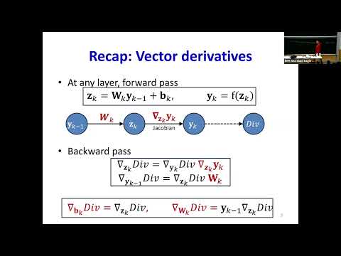
Backpropagation travels backward through this dependency chain, multiplying by activation Jacobians and weight matrices.
Vector notation makes the repeated backward calculation systematic rather than requiring a separate scalar derivation for every unit.

16:45 The Weight-Gradient Rule and Backpropagation’s Role

The derivative for a weight uses the input to that weight and the derivative arriving at its output.
Backpropagation computes derivatives; it is not itself the training algorithm or parameter-update rule.
The lecture transitions from derivative calculation to whether optimizing a chosen loss produces the desired classifier.

18:08 Proxy Losses, Perceptrons, and Outlier Sensitivity

A hard 0-or-1 classifier provides little gradient information, so training uses a continuously varying proxy objective.
A perceptron can find a separating line for separable data, but adding one outlier may radically change its boundary.
Gradient descent on a smooth proxy may barely react to a single point, preferring a stable solution even if it leaves that point misclassified.

22:48 Why a Neural Network May Prefer Stability to Perfect Separation

The same trade-off applies to nonlinear networks: a classifier may make a small adjustment rather than twist around one added example.
The lecture describes perceptron solutions as low-bias but high-variance, while proxy-loss training can have higher bias and lower variance.
Minimizing a differentiable loss does not guarantee minimizing classification error, because the proxy and classification accuracy are different objectives.

25:16 Saddle Points and Local Minima in Neural-Network Losses

A complicated neural-network loss surface may contain many local minima and regions with gradients near zero.
For large networks, the lecture presents saddle points—minima in some directions and maxima in others—as common near-zero-gradient locations.
It notes the hypothesis that many large-network local minima have similar loss values, while stressing that behavior is less clear for small networks.

30:51 Convexity and Three Types of Optimization Behavior

A function is convex when the line segment between any two points on its graph lies on or above the function; a convex set contains every segment between its points.
Convex optimization offers more tractable guarantees than a neural network’s generally nonconvex loss surface.
An iterative method may converge, jitter around a solution, or diverge by moving progressively farther away.

33:00 Learning-Rate Bounds for a One-Dimensional Quadratic

For f(x) = ½ax² + bx + c with a positive, the minimum is at x = −b/a and the second derivative is a.
Gradient descent reaches the minimum in one step when the learning rate is 1/a.
A learning rate between 0 and 2/a converges in this quadratic example; a rate above 2/a causes divergence.

40:54 Anisotropic Curvature Makes One Step Size Difficult

In a two-variable quadratic, different axes can have different curvature and therefore different optimal learning rates.
With curvature 300 along one axis and 1 along another, the corresponding one-step rates are 1/300 and 1.
A rate suited to the shallow direction can diverge along the steep one, while a rate suited to the steep direction makes progress painfully slow along the shallow one.

49:32 Hessian Conditioning and Curvature Normalization

Gradient descent is fastest when curvatures are similar across directions; the ratio between the steepest and shallowest directions makes optimization harder.
A local quadratic approximation uses the Hessian, the matrix of second derivatives, to describe curvature across parameters.
Newton’s method and BFGS use the Hessian or an approximation to it to rescale directions, but a billion-parameter model makes forming and inverting a billion-by-billion Hessian impractical.

51:50 Learning-Rate Schedules for Escaping and Converging

A large initial learning rate can help escape a nearby local minimum, while gradually reducing it can support convergence later.
The lecture describes linear, inverse-iteration, inverse-square, and exponential decay schedules.
A practical alternative is to hold the rate fixed until loss stagnates, then reduce it by a factor and continue.

59:54 Why Adaptive Per-Parameter Learning Rates Are Appealing

A single global learning rate forces every parameter direction to use the same step size despite different curvatures.
Using a separate rate for each of a billion parameters would require tracking and tuning a billion changing values.
Rprop is introduced as a way to adapt steps using local directional information without computing a full Hessian.

1:05:11 Rprop Uses Gradient Signs to Adapt Each Step

Resilient propagation (Rprop) uses the sign of each derivative, not its magnitude, and updates each parameter independently.
When consecutive derivatives have the same sign, Rprop increases that parameter’s step by a factor greater than one.
When the sign flips, indicating an overshoot, Rprop returns to the earlier estimate and reduces the step by a factor below one; step-size ceilings and floors prevent extreme values.

1:14:55 Rprop Caveats and Quickprop’s Curvature Approximation

Rprop still requires backpropagation to determine gradient signs, but it does not use gradient magnitudes or second derivatives.
Its independent coordinate updates can work on nonconvex losses, though pathological or noisy surfaces can cause repeated rollbacks.
Quickprop, developed by Scott Fahlman, estimates second-order information from derivative changes between adjacent iterations rather than computing a full Hessian.

1:16:14 Momentum Averages Gradients to Reduce Oscillation

The lecture revisits trajectories where updates oscillate across a steep direction but move consistently along a shallow direction.
A running average preserves a large update in the consistent direction while positive and negative gradients cancel in the oscillating direction.
Momentum combines the current gradient step with a fraction of the previous step, improving progress without requiring a separate Hessian for each parameter.

1:24:36 Nesterov Acceleration and the Optimization Takeaways

Standard momentum applies the current gradient and then adds the previous-step contribution; Nesterov momentum first advances by the previous-step contribution and evaluates the gradient at the new location.
The lecture presents Nesterov’s accelerated method as a faster alternative to standard momentum on differently curved loss surfaces.
The closing summary highlights adaptive or decaying learning rates, dimension-wise step handling, and momentum as improvements over vanilla gradient descent.

Summary, takeaways, and chapters were generated by AI from the video's transcript and may contain errors. The video belongs to its creator, Carnegie Mellon University Deep Learning.