CMU Introduction To Deep Learning 11-785, Fall 2026: Lecture 5

Overview

Lecture 5 develops backpropagation as repeated applications of the chain rule: a forward pass stores each layer’s affine values and activations, and a backward pass propagates derivatives to compute parameter gradients. It connects those gradients to gradient descent on average training-set divergence, then recasts the calculations in vector and matrix form, including Jacobians, softmax cross-effects, and subgradients for ReLU and max.

Key takeaways

Gradient descent updates a parameter opposite its loss derivative: decrease a weight when increasing it raises loss, and increase it when increasing it lowers loss.
Backpropagation is a derivative-computation procedure, not the learning rule; gradient descent uses the derivatives that backpropagation produces.
The forward pass must retain intermediate activations and affine values because activation derivatives are evaluated at those values during the backward pass.
For a connection with source activation y and destination affine value z, the weight gradient is the z derivative multiplied by y; the bias gradient is the z derivative.
Vector activations such as softmax require summing derivative contributions across outputs, unlike independent scalar activations whose Jacobian is diagonal.
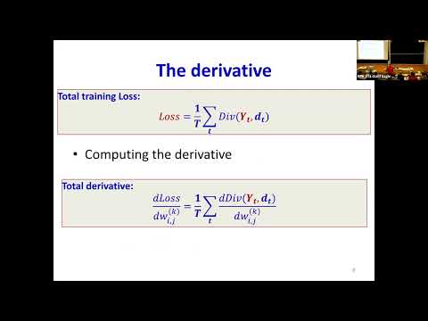
For average training loss, the full-batch gradient is the average of each training example’s divergence gradient before applying the parameter update.

Chapters

0:00 Attendance, Pokémon Roll Call, and Course Expectations

The class is asked to complete an attendance poll and prepare name tags.
Starting with the next class, students will be assigned Pokémon names and must respond when called or risk being marked absent.
The instructor says attendance will count toward course points and encourages students to attend to support learning.

6:00 Training Objective: Average Divergence and Gradient Descent

Neural-network training is framed as minimizing loss with respect to weights and biases.
Average divergence on training examples is a proxy for the desired goal: low error across the broader input space.
Gradient descent updates each parameter as its current value minus a learning-rate-scaled loss derivative.

12:00 Influence Diagrams Derive the Chain Rule

A derivative is treated as the local influence of a small input perturbation on an output perturbation.
For a variable with multiple incoming influences, the output change sums each input change multiplied by its partial derivative.
For indirect influence, derivatives multiply along a path; when several paths connect variables, their contributions sum.

21:00 Checkpoint on Chain-Rule Paths and Network Notation

The class reviews that the chain rule follows from the definition of derivatives and influence diagrams expose the relevant variable paths.
The derivative between two variables sums contributions over every path connecting the influencer to the influenced variable.
The example network uses layer indices plus neuron indices to distinguish weights, affine values, and activation outputs.

24:00 Layered Network Variables: Weights, Biases, z, and y

A weight’s two subscripts identify its source and destination neurons, while its superscript identifies the destination layer.
Each neuron computes an affine value z, then applies an activation to produce output y.
Biases can be represented by adding a constant-one input, allowing the bias to be treated as an ordinary weight.

28:00 Forward Pass Computes Every Layer’s Activations

The input is designated as layer zero, and each neuron’s z is the weighted sum of outputs from the preceding layer.
Each z passes through its activation function to produce y; repeating this computation yields the network output.
A forward pass stores intermediate z and y values needed to evaluate derivatives at the current example and parameter values.

32:00 Backpropagation Starts at the Output and Moves Backward

After comparing the network output with the desired output, the divergence provides the starting point for derivative calculations.
Backpropagation moves from the output toward the input, tracking how perturbations to intermediate values and parameters affect divergence.
The same process can continue to the input, yielding derivatives that describe how input changes affect the output or loss.

36:00 Three Local Derivative Rules Build Scalar Backpropagation

For an activation y=f(z), the divergence derivative with respect to z is the derivative with respect to y multiplied by the activation derivative.
When a variable affects several downstream values, its derivative sums the contributions from all those paths.
For z containing a term y·w, the local derivatives are ∂z/∂y = w and ∂z/∂w = y.

42:00 Backward Recurrence and Per-Weight Gradient Cost

A weight gradient is the derivative of divergence with respect to its destination z, multiplied by the source activation y.
A neuron’s activation-output derivative is a weighted sum of downstream z derivatives; multiplying by the activation derivative gives its z derivative.
The backward pass resembles the forward pass but also computes a gradient for every weight, which adds substantial computation.

49:00 Softmax Cross-Derivatives, ReLU, and Max Subgradients

With scalar activations, each z affects one y; with vector activations such as softmax, a z can affect every output, so derivatives sum across outputs.
Softmax diagonal derivatives are yᵢ(1−yᵢ), while off-diagonal derivatives are −yᵢyⱼ, reflecting competition between output probabilities.
ReLU is nondifferentiable at zero; a subgradient can take any value from 0 to 1 there, and the lecture describes choosing 1.
For max(x₁, x₂, x₃) with x₁ uniquely largest, the local derivative is 1 for x₁ and 0 for the other inputs.

1:00:00 Average Per-Example Gradients for Gradient Descent

For each training example, the forward pass stores the intermediate z and y values and the backward pass computes divergence derivatives.
Because the loss is average divergence over training examples, its parameter gradient is the average of the per-example gradients.
The resulting average gradient is inserted into the gradient-descent update for each network parameter.

1:03:00 Vectorized Forward Pass: z = Wy + b

All neuron affine values in a layer form a vector z, and outputs from the preceding layer form a vector y.
Combining the individual weighted sums yields the layer equation zₖ = Wₖyₖ₋₁ + bₖ, followed by yₖ = activationₖ(zₖ).
Vector notation makes the forward-pass implementation concise and supports efficient matrix operations on GPUs.

1:08:00 Vector Derivatives and Jacobian Dimensions

The perturbation rule extends to vectors: δy equals the derivative of y with respect to x multiplied by δx.
If y has m components and x has n components, the derivative is an m-by-n Jacobian so the perturbation dimensions align.
Influence diagrams and chain-rule reasoning remain applicable to vector-valued functions, provided matrix multiplication order is tracked.

1:13:00 Matrix Parameter Gradients for Weights and Biases

For z = Wy + b, the derivative of z with respect to b is an identity matrix, so the bias gradient follows directly from the z derivative.
The weight gradient combines the source activation y with the derivative of divergence with respect to z; its matrix shape must match W.
The lecture emphasizes checking dimensions and transpose conventions when moving between scalar, vector, and matrix derivatives.

1:18:00 Stacked Jacobians Represent Layer Activations

A vector output’s Jacobian can be understood as stacking the derivatives of its individual scalar outputs.
For independent scalar activations, the activation Jacobian is diagonal because each z affects only its corresponding y.
For vector activations such as softmax, off-diagonal Jacobian entries capture cross-output influence.

1:22:00 Matrix Backpropagation Alternates Jacobians and Weight Matrices

Backpropagation begins with the divergence derivative at the network output and applies the output activation Jacobian to obtain the final z derivative.
Moving backward alternates activation Jacobians with weight matrices, propagating derivatives one layer at a time.
At each layer, the bias gradient comes from the z derivative and the weight gradient combines that derivative with the preceding layer’s activation.

1:26:00 Training Pipeline and Preview of Generalization

Classification labels can be represented as one-hot vectors, while the network output may be probabilities or real-valued predictions for regression.
The full training recipe combines forward passes, backward-pass gradients, averaging across examples, and gradient descent.
The next class is scheduled for Friday from 8:00 to 9:20 and will address learning, generalization, and the meaning of network outputs.

Summary, takeaways, and chapters were generated by AI from the video's transcript and may contain errors. The video belongs to its creator, Carnegie Mellon University Deep Learning.