CMU Introduction To Deep Learning 11-785, Fall 2026: Lecture 13

Overview

Bhiksha Raj introduces recurrent neural networks by contrasting finite-window CNNs with models that carry information across time, then traces the progression from output-feedback networks and Jordan and Elman networks to state-space RNNs. He explains unrolling, shared weights, sequence-level losses, and backpropagation through time (BPTT), then closes with bidirectional RNNs and why their use depends on whether future inputs are available.

Key takeaways

A time-delay CNN has finite temporal memory: an input affects predictions only while it remains inside the model’s fixed history window.
NARX-style output feedback extends influence across time, but can bottleneck history in the output; an RNN instead carries prior computation in its hidden state.
The Elman network’s copied context unit carries information forward but blocks gradient flow through the copy, unlike a fully recurrent state-space model.
BPTT treats an RNN as one unrolled, shared-parameter network: gradients flow backward through time and accumulate across every use of each weight.
Bidirectional RNNs combine past and future context by concatenating two directional hidden states, but require the complete sequence and therefore are unsuitable for decisions that depend on unavailable future data.

Chapters

0:00 Classroom Setup and Attendance Poll

The opening minutes include classroom setup and informal conversation before the lecture begins.
At about 5:42, Bhiksha Raj asks students to open the attendance poll and put phones and laptops away.

7:30 Why Speech, Text, and Markets Need Sequence Models

Speech recognition maps a series of spectral vectors to a transcript, while sentiment analysis may need the complete text before producing one label.
A Pittsburgh Steelers news excerpt illustrates that readers infer football from contextual clues such as an average of 30 points allowed per game.
Machine translation and stock prediction likewise map input sequences to a single output or a sequence of outputs.

13:45 CNN Time Windows Create Finite-Response Models

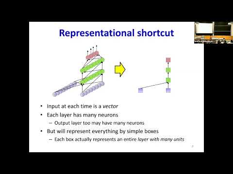
Bhiksha Raj introduces a compact diagram convention: each box represents a vector or layer, and each arrow denotes full connectivity between its endpoint layers.
A time-delay CNN predicts from a finite window of past stock values, so an event stops affecting predictions after it leaves the window.
Expanding the window increases the model and its parameter count, while useful trends may span daily, weekly, monthly, seasonal, and annual cycles.

18:10 Autoregressive Output Feedback Gives History a Long Tail

An infinite-response model should let an event influence future outputs while its effect fades over time—for example, comparing several past Christmas seasons.
In a nonlinear autoregressive model with exogenous inputs (NARX), the current output is fed back alongside later inputs to produce subsequent outputs.
The feedback can carry influence forward indefinitely, but the history is compressed into the output rather than stored in the network’s internal computation.

20:15 Jordan Memory and Elman Context Units

Michael I. Jordan’s network uses a running, exponentially weighted memory of past outputs; this still stores history through outputs rather than internal computation.
The Elman network copies a hidden state into a context unit and supplies that value as an extra input at the next time step.
Because the Elman context is copied without a derivative connection, current errors cannot backpropagate through the copy to earlier computations.

27:05 State-Space RNNs Make Hidden State Truly Recurrent

A state-space model updates hidden state as h_t = f(x_t, h_{t-1}) and computes the output from h_t.
The hidden state is intended to summarize past inputs and computations, so an event can affect outputs long after it occurs.
The initial state, such as h_{-1}, must be specified; it may be fixed or learned.

44:30 Multi-Step Recurrence and Time-Unrolled Diagrams

Allowing a hidden state to depend on states from multiple earlier steps can represent more complex temporal patterns than one-step recurrence.
A k-step recurrence requires k initial hidden-state values; Bhiksha Raj notes the added complexity as a reason to focus on one-step models.
The looped arrows in common RNN diagrams represent connections across time, not a layer feeding back into itself within one time step.

49:30 RNN Equations Separate Current and Recurrent Weights

For a single hidden layer, the pre-activation combines the current input, the previous hidden state, and a bias before applying an activation.
Input-to-hidden weights are current weights; hidden-to-hidden weights carry information from the previous time and are recurrent weights.
In multilayer RNNs, each vertical or within-time connection and each across-time connection has its own parameter set.

53:20 RNN Input-Output Patterns for Captioning and Translation

A single image input can initialize hidden states that generate a caption over multiple time steps.
Sentiment analysis and the Steelers example can read a full input sequence before producing one final output.
Machine translation reads one language sequence and generates another; the general sequence-to-sequence pattern can also produce outputs at each input step.

57:30 Sequence Training Shares One Network Across Time

Each training example contains an input sequence and a desired output sequence, and the RNN produces an output sequence for comparison.
Unrolling the RNN reveals repeated copies of the same network with shared parameters across time steps.
The forward pass processes the sequence using the current input and prior hidden state, then applies an activation such as tanh.

1:01:10 Sequence Losses and the Alignment Problem

Training requires a differentiable divergence between the predicted output sequence and the target sequence.
In tasks such as speech recognition or machine translation, predicted and target word sequences may have different lengths and no direct one-to-one alignment.
When outputs do align step by step, the sequence loss can be formed from local losses; later methods address cases without that correspondence.

1:06:30 BPTT Applies the Chain Rule Across Time

Backpropagation through time (BPTT) sends gradients backward through the unrolled computation, opposite the forward sequence pass.
The derivation uses standard chain-rule operations: activation Jacobians, connection weights, and input-times-error terms for weight gradients.
The sequence-level loss must provide a derivative with respect to each output before those gradients can propagate through the RNN.

1:13:00 Recurrent Gradients Accumulate for Shared Parameters

A hidden state that feeds both the next layer and the next time step receives gradient contributions from both paths, which must be summed.
Each shared weight accumulates gradient contributions from every time step where that parameter is used.
The network parameters remain fixed during one complete forward and backward pass; an optimizer update happens after gradient computation.

1:20:30 Train on Complete Sequences, Not One Vector at a Time

An RNN training example is an entire input sequence paired with an output sequence, rather than one independent vector.
The model processes the sequence before computing its loss and updating parameters; it does not update after every vector.
Sequences can have different lengths, although implementation and memory constraints may motivate fixed-size batches.

1:22:30 Bidirectional RNNs Add Future Context

Part-of-speech tagging can benefit from future words as well as past words when deciding whether a word is a noun or adjective.
A bidirectional RNN uses separate forward and backward networks, then concatenates their hidden states at each time step.
It suits tasks with access to the full input, such as offline speech or text processing, but not day trading decisions that cannot use future market data.

1:25:30 Backpropagation Through Forward and Backward RNNs

At each time step, the gradient of the concatenated hidden state splits into forward-state and backward-state components.
BPTT traverses the forward network in reverse temporal order and the backward network in the reverse of its own processing order.
Gradients reaching the shared input are summed across both directional networks before propagating to earlier layers.

Summary, takeaways, and chapters were generated by AI from the video's transcript and may contain errors. The video belongs to its creator, Carnegie Mellon University Deep Learning.