CMU Introduction To Deep Learning 11-785, Fall 2026: Lecture 11
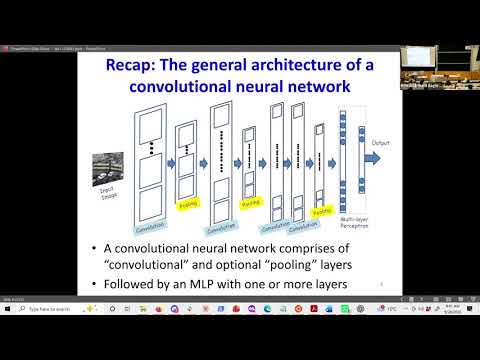 Watch on YouTube →
Overview
The CMU 11-785 lecture derives backpropagation through CNN convolution and pooling layers, connecting the chain rule to practical tensor operations. It shows how input gradients use spatially flipped filters and padding, filter gradients use input and output-gradient maps, and max/mean pooling redistribute gradients according to which inputs contributed.
Key takeaways
- A convolutional input element can affect several output positions and channels, so its gradient sums the corresponding output gradients weighted by the filter elements that connected them.
- For input gradients, spatially flip the filters and pad output-gradient maps as needed; the backward result must match the original input’s dimensions.
- For a filter weight, the local derivative is the input value paired with it in the forward pass, and its total gradient sums that value times the output gradient across all uses.
- Max-pooling backpropagation routes gradients to recorded argmax locations, while mean-pooling backpropagation divides each gradient evenly among the window’s inputs.
- Overlapping pooling windows can send multiple contributions to one input location, so backward code must accumulate gradients rather than overwrite them.
- Reverse-mode differentiation can be implemented by traversing the forward computation in reverse and applying local derivative rules for activations and products.
Chapters
0:00
Before Class: Room Chatter and a Slides Upload Delay
- Informal pre-class conversation includes travel routes involving Pittsburgh, Los Angeles, Chicago, and Dallas.
- At 9:08, attendance polling begins; a GitHub merge/push issue briefly delays access to the lecture slides.
9:08
CNN Recap: Pattern Scanning and Position Invariance
- CNNs address pattern-classification tasks such as identifying a cat in an image or “hello” in a recording by scanning for targets.
- The recap distinguishes 2D-or-higher-dimensional CNNs from 1D CNNs, also called time networks.
12:00
Convolution Filters Combine Input Channels into Output Maps
- Each convolution filter spans every input channel and a local spatial patch; a 3×3 example computes a weighted inner product plus a bias.
- Each filter produces one output channel, so the number of filters equals the number of output maps.
- An activation function is applied pointwise to the affine map, while each affine output depends on all input channels.
16:30
Pooling, Strides, and CNN Resizing Operations
- Max pooling selects and records the largest value in each window; mean pooling outputs the window average.
- Downsampling by a factor of two discards every second row and column, while upsampling inserts zeros between map elements.
- Downsampling can be combined with a preceding operation through stride; zero insertion is useful when followed by convolution, sometimes described as fractional-stride convolution.
20:30
Training CNNs and Passing Gradients Back from the MLP
- CNN training follows the standard supervised-learning loop: compute outputs, compare them with target labels using a loss, and use gradient descent.
- For a batch, the loss and its gradient are averages over the individual training examples.
- The final convolutional maps are flattened into a vector for an MLP; backpropagating through that MLP yields gradients that can be reshaped to the map dimensions.
25:00
Backpropagating Through a Convolutional Activation
- The convolution layer is treated as two operations: an affine map followed by a pointwise activation.
- For each location, the gradient with respect to the affine value equals the output gradient multiplied by the activation-function derivative at that value.
- This chain-rule step supplies the affine-map gradients needed to continue backward through the convolution.
29:00
Tracing How One Input Pixel Affects Many CNN Outputs
- A single input-map element can contribute to multiple positions in each output map because the filter scans across the input.
- Its gradient therefore sums contributions from every affected output position and every output channel.
- The filter channel connecting a particular input map to an output map determines the weight used in each contribution.
33:00
Convolution Indices Explain the Input-Gradient Rule
- With the lecture’s indexing convention, an input element at (x, y) contributes to output (x′, y′) through filter element (x−x′, y−y′).
- The derivative of that output with respect to the input element is the corresponding filter weight.
- Summing these weighted output gradients gives the gradient for each input location.
38:00
Input Gradients Use Flipped Filters and Zero Padding
- Computing an input gradient can be visualized as convolving the output-gradient map with the filter flipped top-to-bottom and left-to-right.
- Padding the output-gradient map with zeros lets the backward operation produce a gradient with the same spatial size as the original input.
- For an input size M and filter size L in a valid convolution, the forward output has size M−L+1; padding is needed to restore size M during backpropagation.
43:00
Transpose Convolution Accumulates Gradients Across Channels
- To compute one input channel’s gradient, take that channel from every output filter, flip the spatial filter dimensions, and combine the resulting convolutions with output-channel gradients.
- The filter’s channel and spatial indices are rearranged in the backward operation, motivating the name transpose convolution.
- The lecture emphasizes checking that the resulting gradient has the same dimensions as the input to the forward operation.
48:00
Channel Selection and Padding in Convolution Backpropagation
- For a chosen input channel, only the corresponding channel slices from all filters are needed to compute its gradient.
- Output-gradient maps are zero-padded before applying the flipped filters so that edge and interior input positions receive the correct contributions.
- If the forward convolution used zero padding, the backward computation must account for that padded input shape as well.
53:00
Completing the Input-Gradient Calculation
- The backward computation combines the relevant filter slices with gradients from all output maps, accumulating contributions for each input channel.
- The lecture presents convolution as the practical operation underlying this calculation, while noting that real implementations process the maps as tensors on a GPU.
- A classroom poll reviews the channel selection, filter flipping, and convolution steps before moving to filter gradients.
59:00
Deriving Gradients for Individual Filter Weights
- A filter element affects multiple output positions because the filter is reused at every scan location.
- For output location (x, y) and filter element (i, j), the forward contribution uses the input at (x+i, y+j).
- Consequently, the derivative of that output with respect to the filter element is the corresponding input value.
1:04:00
Summing Filter-Weight Gradients Across Output Positions
- The gradient for a filter element sums over all output-map positions where that weight was used.
- Each term multiplies the output-gradient value by the input element that paired with the weight in the forward pass.
- A filter belongs to one output channel, and each of its channel slices operates on one input channel.
1:09:00
Filter Gradients as Input–Output-Gradient Convolutions
- To compute a filter-channel gradient, align the relevant input map with the output-gradient map and scan to form the required inner products.
- Unlike the input-gradient calculation, this filter-gradient operation does not flip the filter or require the same zero-padding step.
- The lecture notes that forward-pass zero padding must still be represented when deriving gradients for padded inputs.
1:14:00
Reverse-Mode Differentiation Directly from Code
- The lecture reduces backpropagation to local rules for unary activations and binary products, then applies those rules in reverse computation order.
- For an activation y=σ(z), the local rule is to multiply the incoming gradient by σ′(z); for a product, gradients use the other multiplicand.
- In the convolution loops, reverse the layer and position traversal and accumulate contributions with plus-equals wherever multiple paths reach the same variable.
1:20:00
Max and Mean Pooling Gradients, Plus a Shape Check
- Max pooling sends the gradient only to the stored argmax location in each window; all other locations receive zero.
- Overlapping max-pooling windows require gradient accumulation, and the lecture recalls a PyTorch issue caused by failing to add overlapping contributions.
- Mean pooling distributes the output gradient uniformly across the window, multiplying each input contribution by 1 divided by the window size.
- At every backward operation, the gradient must account for every input element that influenced the output; the instructor confirms that max-pooling backward uses the argmax recorded during the forward pass.
Summary, takeaways, and chapters were generated by AI from the video's transcript and may contain errors. The video belongs to its creator, Carnegie Mellon University Deep Learning.