Building makemore Part 3: Activations & Gradients, BatchNorm

Overview

Andrej Karpathy delves into neural network initialization and activation/gradient behavior, highlighting how poor initialization leads to high initial loss and "hockey stick" loss curves. He demonstrates fixing these issues by adjusting weights and biases to achieve expected initial loss and better activation distributions, ultimately improving training performance and reducing saturation in activation functions like Tanh. The lecture also introduces Batch Normalization as a modern technique to stabilize training in deeper networks by normalizing activations, though it introduces complexities like batch coupling and requires careful handling during inference.

Key takeaways

Poor neural network initialization leads to high initial loss and 'hockey stick' loss curves, fixable by scaling weights and zeroing biases.
Saturated activations (e.g., in Tanh) cause gradient vanishing; scaling weights by `gain / sqrt(fan_in)` (e.g., 5/3 for Tanh) stabilizes activations and gradients.
Batch Normalization normalizes activations across batches, stabilizing training in deep networks and reducing sensitivity to weight initialization, but introduces batch coupling.
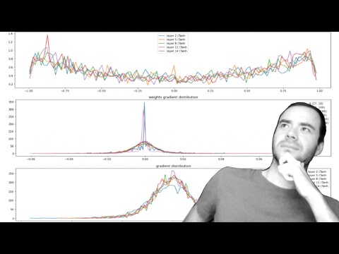
Diagnostic plots of activation/gradient histograms and update-to-data ratios are essential for understanding network behavior and debugging training issues.
The update-to-data ratio, ideally around 1e-3 (log scale -3), helps calibrate learning rates and diagnose slow or unstable training.

Chapters

0:00 Introduction: Moving Beyond MLP for Character-Level Language Modeling

Continuing the 'makemore' implementation from the previous lecture on MLP for character-level language modeling.
Goal: Understand activations and gradients in neural nets during training, crucial for RNNs and their variants.
Focus on intuitive understanding of gradient flow and activation behavior to explain optimization challenges in RNNs.

2:03 Code Refactoring and Baseline MLP Performance

Code cleaned up from previous lecture, removing magic numbers by defining embedding dimensionality and hidden unit counts.
MLP with 11,000 parameters trained for 200,000 steps with a batch size of 32.
Observed training and validation loss around 2.16, with refactored evaluation and sampling functions.

5:04 Understanding torch.no_grad Decorator

Decorator used for evaluation functions to disable gradient computation.
Informs PyTorch not to track operations for backpropagation, improving efficiency.
Tensors within a `no_grad` context have `requires_grad=False`.

6:34 Initial Model Sampling and Word Generation Quality

Sampling from the model produces slightly improved, more name-like words compared to the previous BAM model.
Model still not perfect, but generation quality shows progress.
Demonstrates the output of the current MLP model's sampling capability.

7:00 Problem 1: Poor Initialization and High Initial Loss

Observed initial loss of 27 on the zeroth iteration, indicating improper network configuration.
Expected initial loss calculated as -log(1/27) ≈ 3.29, significantly lower than observed.
High initial loss caused by the network confidently predicting incorrect characters with extreme logit values.

10:11 Illustrating Extreme Logits and High Loss

Example with 4 characters: logits near zero produce a uniform distribution (loss 1.38).
Extreme positive or negative logits lead to confident, incorrect predictions and very high loss.
Normally distributed logits scaled by 10 can result in extremely high losses.

14:07 Fixing Initialization: Zeroing Bias and Scaling Weights

Bias B2 initialized to zero to avoid random offsets in logits.
Weight matrix W2 scaled down (e.g., by 0.01) to reduce logit magnitudes.
Scaling W2 by 0.01 brings initial loss closer to the expected 3.29, with slight entropy for symmetry breaking.

18:38 Impact of Improved Initialization on Training

Training with corrected initialization shows no initial 'hockey stick' loss curve.
Optimization spends less time squashing overly large weights, leading to more productive training cycles.
Validation loss improved from 2.16 to approximately 2.13.

21:40 Problem 2: Saturated Tanh Activations

Even with corrected logits, hidden state activations (H) are problematic.
Histogram of H shows most values are at -1 or 1, indicating saturation of the Tanh function.
Pre-activation values feeding into Tanh have a broad distribution, causing Tanh outputs to cap at -1 and 1.

25:15 Gradient Vanishing in Tanh's Flat Regions

Tanh's local gradient is `1 - T^2`, which is near zero when T is close to -1 or 1.
When activations are saturated, gradients are killed, preventing learning in those neurons.
Visualizing 'flat region' activations (> 0.99) shows widespread saturation, though no 'dead neurons' (entire columns white) were observed.

33:43 Dead Neurons and Non-linearities (ReLU, Sigmoid)

A 'dead neuron' occurs when its output is always saturated, preventing gradients from flowing.
Sigmoid and ReLU also suffer from flat regions (ReLU below zero) that can lead to dead neurons.
Dead ReLU neurons never activate, their weights and biases never learn.

39:59 Fixing Tanh Saturation: Scaling Weights

Pre-activation values (H_preact) are too extreme, causing Tanh saturation.
Scaling W1 by 0.1 reduces the range of H_preact, leading to a better histogram and less saturation.
Further adjustment to W1 scaling (e.g., 0.2) improves the distribution of pre-activations.

42:29 Impact of Tanh Saturation Fix on Training

Training with improved initialization (scaled W1) results in a validation loss of 2.10.
This is an improvement over the initial 2.17 and the 2.13 after fixing softmax confidence.
Better initialization allows more productive training cycles by avoiding gradient vanishing.

46:53 Principled Weight Initialization: Scaling by Fan-in

Motivation: Avoid manual 'magic numbers' for scaling weights.
Analysis of `X @ W`: input standard deviation (1) expands to 3 after multiplication.
To preserve standard deviation, scale weights by `1 / sqrt(fan_in)`.

52:21 Kaiming Initialization and Gain Factors

Kaiming et al. paper ('Delving Deep into Rectifiers') analyzes ReLU and other non-linearities.
For ReLU, weights are initialized with std dev `sqrt(2 / fan_in)`.
For Tanh, the advised gain is `5/3` on top of `1 / sqrt(fan_in)` due to its contractive nature.

1:02:20 Implementing Kaiming Initialization for Tanh

Target standard deviation for weights: `gain / sqrt(fan_in)`.
For Tanh, gain is 5/3. Fan-in for W1 is 30 (embedding_dim * block_size).
Calculate scale factor: `(5/3) / sqrt(30) ≈ 0.304`, applied to W1 initialization.

1:06:44 Training with Kaiming Initialization

Training with Kaiming initialization yields validation loss of 2.10, comparable to previous results.
Eliminates need for manual scaling, providing a principled approach.
Modern innovations have made precise initialization less critical, but understanding remains valuable.

1:07:26 Introduction to Batch Normalization

Batch Normalization (BN) introduced in 2015 stabilizes training of deep networks.
Insight: Normalize hidden states to have zero mean and unit variance (Gaussian distribution).
Standardizing activations is a differentiable operation.

1:10:47 Batch Normalization Mechanism: Standardization

Calculate mean and variance across the batch for each neuron's pre-activations (H_preact).
Standardize H_preact by subtracting mean and dividing by standard deviation.
This ensures each neuron's output is unit Gaussian for the current batch.

1:16:39 Batch Normalization: Scale and Shift (Learnable Parameters)

Introduce learnable gain (gamma) and bias (beta) parameters after standardization.
BN gain initialized to 1, BN bias to 0, preserving unit Gaussian output at initialization.
Gamma and beta allow the network to learn optimal scaling and shifting of activations.

1:19:04 Batch Normalization Impact on a Simple Network

Training with BN on a single-hidden-layer MLP yields validation loss of 2.10.
Little improvement in this simple case because manual scaling already produced good results.
BN becomes crucial for deeper, more complex networks where manual tuning is intractable.

1:23:37 Batch Normalization's Cost: Batch Coupling

BN couples examples within a batch, making activations dependent on batch statistics.
This 'jitter' acts as a regularizer, similar to data augmentation, preventing overfitting.
This coupling is undesirable and leads to bugs, motivating alternatives like Layer Normalization.

1:30:02 Handling Batch Normalization at Inference Time

Problem: BN requires batch statistics, but inference uses single examples.
Solution 1: Calibrate BN by estimating mean/variance over the entire training set after training.
Solution 2 (preferred): Maintain running mean/variance during training using exponential moving average.

1:38:51 Running Mean/Variance Update in Batch Normalization

Running mean/variance updated using exponential moving average (e.g., momentum 0.999).
Updates are done outside gradient-based optimization using `torch.no_grad()`.
This avoids a second calibration stage and allows single-example inference.

1:41:40 Batch Normalization Implementation Details

Epsilon added to denominator to prevent division by zero if batch variance is zero.
Bias in preceding linear layers becomes redundant and is typically removed when followed by BN.

1:45:08 Summary of Batch Normalization Layer

Controls activation statistics, typically placed after linear/convolutional layers.
Has learnable gain/bias parameters and buffers for running mean/variance.
Normalizes batch, then scales/shifts using learned parameters; maintains running stats for inference.

1:47:30 ResNet Architecture and BN Placement

ResNet uses repeating blocks with Convolution, Batch Normalization, and ReLU (Conv-BN-ReLU motif).
Convolutional layers are like linear layers applied to patches of input.
Bias is disabled in Conv layers preceding BN, similar to linear layers.

1:55:01 PyTorch Linear and BatchNorm Layer Details

PyTorch `nn.Linear` initializes weights using `1/sqrt(fan_in)` (uniform distribution by default).
`nn.BatchNorm1d` takes features, epsilon, momentum; uses learnable gamma/beta and running stats.
Momentum value affects running stats update; smaller batch sizes may need lower momentum.

Summary, takeaways, and chapters were generated by AI from the video's transcript and may contain errors. The video belongs to its creator, Andrej Karpathy.