6:1 Conservation of Mass - Frames of Reference, Material Derivatives, Convective Acceleration

Overview

Derek Elsworth connects conservation laws to fluid-flow analysis, moving from Bernoulli and continuity examples to reference frames and the material derivative. He shows how a fixed observer can infer the acceleration experienced by a moving fluid particle, then applies that idea to temperature logs and Newton’s second law, setting up later work on conservation of mass, momentum, and energy.

Key takeaways

For a constant-density stream tube, continuity requires A₁v₁ = A₂v₂; as a falling jet accelerates under gravity, its cross-sectional area decreases.
Bernoulli’s free-jet result v = √(2gH) relates outlet speed to elevation drop when the tank surface speed is negligible and both points are at atmospheric pressure.
A moving logging tool measures temperature change along its trajectory; combining that measurement with tool speed and a spatial temperature gradient separates temporal change from advective change.
The material derivative D/Dt = ∂/∂t + u∂/∂x + v∂/∂y + w∂/∂z captures particle acceleration even when a steady flow has no local time variation.
For the steady field u = 2x, v = −y, w = z, convective acceleration is (4x, y, z), demonstrating that spatial variation alone can accelerate fluid particles.
A Pitot tube facing upstream registers hydraulic pressure head plus velocity head, whereas a piezometer measures the hydraulic grade without that velocity contribution.

Chapters

0:00 Course Roadmap: Conservation Laws, Moving Frames, and Borehole Logs

Elsworth previews three conservation topics: mass balance, momentum through Newton’s second law, and energy including real-flow losses.
A boat moving at 1 m/s while a cannon ejects water forward at 1 m/s gives a 2 m/s water speed to a stationary observer.
Borehole tools such as gamma, resistivity, and spinner logs record properties over time as they travel, although the desired profile is by depth.

5:50 Exam Feedback and the Week-Six Course Checkpoint

Elsworth reports that scores resemble previous years, with many A grades and roughly 98% of students reaching the grade needed to continue.
He recommends using past exams to identify likely problem formats and practise the associated methods.
The class is about one-third through a 15-week semester and is moving from Bernoulli applications into conservation equations.

8:28 Bernoulli Applications: Jet Lab Support and Aerodynamic Drag

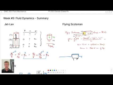
For the jet-lab example, Bernoulli relates a pressurized upstream point to an atmospheric jet; Elsworth cites a flow requirement of about 14 kW and a jet speed near 100 m/s.
The SFO tarmac and Flying Scotsman examples use pressure differences to estimate forces on an object in moving air.
At 30 m/s, the example yields about 450 N of force and 15 kW of power for a 1 m face; a smaller effective area brings the estimate closer to human-scale power.

14:00 Free Jets, Streamlines, and Continuity

Applying Bernoulli between a large tank surface and its outlet gives the free-jet relation v = √(2gH), where H is the elevation drop.
Continuity, A₁v₁ = A₂v₂ for constant-density flow, explains why a falling water stream narrows as its speed increases.
A jet’s horizontal travel distance can be found from horizontal speed multiplied by fall time; vertical motion follows gravity and produces a parabolic path.

21:00 Tank Surface Motion and Bernoulli Head Lines

A large tank’s surface speed can often be approximated as zero, but a smaller tank requires continuity to relate surface velocity to outlet velocity.
Elsworth distinguishes elevation head, pressure head, and velocity head, whose sum forms the energy grade line in ideal Bernoulli flow.
A piezometer indicates hydraulic grade, while a Pitot tube facing upstream also converts velocity head into pressure head.

27:00 Fixed, Translating, and Deforming Control Volumes

A stationary, non-deforming pipe is one reference-frame case; a jet engine moving without changing shape is another.
A moving, deforming control volume, such as an inflating balloon, has a changing volume, expressed as dV/dt ≠ 0.
Mass conservation is framed as mass rate in minus mass rate out equalling the rate of mass accumulation inside a control volume.

32:00 Material Derivative: Converting Borehole Temperature Logs to Spatial Change

For temperature T moving with a logging tool, the material derivative is D T/Dt = ∂T/∂t + v_z ∂T/∂z in the vertical example.
Elsworth uses a geothermal gradient of about 25°C per kilometre and a logging speed of 1 km/h to illustrate a 25°C/h temperature change along the tool’s path.
If the temperature field also rises uniformly by 5°C over an hour, that temporal change adds to the spatial-gradient contribution measured by the moving tool.

40:08 Material Acceleration in Newton’s Second Law

Newton’s second law requires particle acceleration, written as Dv/Dt rather than only the velocity change seen at a fixed location.
In three dimensions, the material derivative adds local time change to advection: ∂/∂t + u∂/∂x + v∂/∂y + w∂/∂z.
For a steady velocity field, the local time-derivative term is zero, but spatial velocity gradients can still produce acceleration.

44:50 Velocity-Field Example and the Need for Convective Acceleration

Elsworth’s example uses velocity components u = 2x, v = −y, and w = z, so speed changes with position even in a steady field.
Applying the spatial terms of the material derivative gives acceleration components (4x, y, z) for that example.
A stationary observer can infer a moving particle’s acceleration from its velocity and how the velocity field changes across space—the basis for applying momentum equations to fluid flow.

Summary, takeaways, and chapters were generated by AI from the video's transcript and may contain errors. The video belongs to its creator, Derek Elsworth.