2026 10 02 Math219 03

Overview

Clark Bray develops the geometric tools for calculus on parametric curves, including position and arc-length differentials, unit tangent vectors, and the curve-length integral. He then defines vector fields through physical examples, connects gradients and inverse-square fields to force and potential conventions, and derives the flux formula for fluid flowing through an oriented area.

Key takeaways

For a parametrized curve r(t), local arc length satisfies ds = ‖r′(t)‖dt, so total length is the integral of speed over the parameter interval.
The identity F(x, y) = (x, y) points radially outward, while F(x, y) = (−y, x) applies a 90-degree counterclockwise rotation at every location.
A radial inverse-square field has the form of a radial unit vector times a 1/r² magnitude; its Cartesian components can obscure this magnitude by displaying an r³ denominator.
Gradients form vector fields, but physical force is commonly F = −∇U; omitting the minus sign reverses the force direction relative to potential energy.
For a uniform fluid velocity F crossing a flat area A with unit normal n, the signed flow rate is Φ = (F · n)A, so motion parallel to the surface contributes no flux.

Chapters

0:00 Parametric Curves: Velocity, Differentials, and the Unit Tangent

The derivative r′(t) is the velocity vector: it is tangent to the curve, points in the direction of motion, and has magnitude equal to speed.
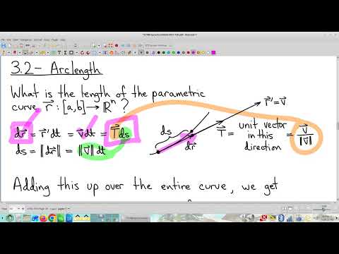
The position differential dr is a linear estimate of position change over a small time interval; it is a vector and may differ from the actual curved displacement.
The arc-length differential ds is a scalar estimate of curve length, with ds = ‖dr‖ = ‖r′(t)‖dt.
The unit tangent T is the normalized velocity, and dr = T ds expresses displacement as direction multiplied by length.

9:09 Computing Parametric Curve Length with Speed Integrals

Total curve length is obtained by adding local lengths: L = ∫‖r′(t)‖dt over the parameter interval.
The integrand is speed, so the formula follows the familiar distance = speed × time relationship applied over many small intervals.
Taking the velocity magnitude commonly introduces a square root; Clark Bray notes that difficult integrals may be assigned without requiring evaluation.
The section also introduces arc-length parameterization as further reading, while emphasizing the length integral as the practical application.

14:06 Vector Fields as Functions from Locations to Vectors

A vector field assigns a vector to every point in its domain, making it a function from ℝⁿ to ℝⁿ with locations as inputs and field vectors as outputs.
Electric, magnetic, and gravitational fields illustrate the physical meaning: each vector records a direction and strength at a location.
Vector-field diagrams are distinct from graphs, level sets, and parametrized curves; each type of picture supports different geometric interpretations.
The broader calculus of vector fields will become central in Chapters 6 and 7, with an initial preview introduced here.

18:40 Constant, Identity, and 90-Degree Rotation Vector Fields

The constant field assigns the same vector, (2, 1), at every point; constancy does not imply a horizontal graph-like picture.
The identity field F(x, y) = (x, y) assigns each location its position vector, drawn with its tail at that location.
The field F(x, y) = (−y, x) rotates each position vector 90 degrees counterclockwise.
The rotation rule is represented by the linear transformation matrix with columns given by the images of the standard basis vectors.

24:57 Radial Inverse-Square Fields and Spherical Coordinates

A radial inverse-square field can be written as a radial unit vector multiplied by a magnitude proportional to 1/r².
The Cartesian-looking numerator over r³ can suggest inverse-cube behavior, but factoring out the unit vector shows that the field magnitude is inverse-square.
Gravitational attraction points inward by using a negative constant, while outward radial fields can model other force configurations.
In spherical coordinates, the radial direction is eᵣ and distance from the origin is ρ, making the field’s structure especially clear.

30:30 Gradients, Anti-Gradients, and the Potential-Energy Sign

A gradient is itself a vector field because it assigns an uphill-pointing vector to every point of a scalar function.
Clark Bray calls a scalar function whose gradient recovers a vector field an anti-gradient, while noting that the more common term is potential function.
For physical forces, force points opposite the gradient of potential energy: F = −∇U.
The sign convention matters: a force field’s potential function may be the negative of physical potential energy, so confusing the terms can reverse the predicted force direction.

37:04 Using Vector Fields to Model Fluid and Animal Movement

A fluid-flow field commonly assigns the local velocity of the fluid to each point in three-dimensional space.
The same model applies to air in a room, ocean currents, and the movement of pollution through air or water.
Zebra migrations can be modeled as a flow when viewed at large scale, where individuals behave like many moving particles with locally coordinated motion.
Fluid-flow interpretations later provide a useful way to reason about electric, magnetic, and gravitational fields.

41:10 Deriving Flux Through an Oriented Surface

The flow through a small area depends on its orientation, which is represented by a unit normal vector n.
Over a time interval Δt, fluid displacement is velocity multiplied by Δt; only its component perpendicular to the surface contributes to crossing it.
The perpendicular displacement is the dot product of displacement with n, and multiplying by area A gives the volume that passes through.
For a uniform field F, the volume flow rate is Φ = (F · n)A, measured in volume per time; Clark Bray introduces Φ as flux and continues the topic in the next class.

Summary, takeaways, and chapters were generated by AI from the video's transcript and may contain errors. The video belongs to its creator, Clark Bray Math.