2026 10 02 Math219 01

Overview

Clark Bray Math builds intuition for vector fields by distinguishing them from graphs and interpreting their arrows through examples: constant vectors, position vectors, 90-degree rotations, and radial inverse-square fields. The lecture connects gradients and potential functions to vector fields, derives flux as flow rate through an oriented surface, defines flow lines through differential equations, and previews the del operator and divergence as a measure of local outward flow.

Key takeaways

A vector field maps each point to an attached vector, not to a graph value; for F(x, y) = (x, y), arrows point radially outward with magnitude equal to distance from the origin.
The field F(x, y) = (-y, x) is a 90-degree counterclockwise rotation of each position vector, and its unit-circle flow line is x = cos t, y = sin t.
For a velocity field crossing a small oriented surface, volume flow rate is the field dotted with the unit normal and multiplied by area; only the perpendicular component crosses the surface.
Using density times velocity as the vector field makes the same flux calculation measure mass flow per unit time instead of volume flow per unit time.
A flow line satisfies the differential equation that the path’s velocity equals the vector field evaluated at the path’s current position.
Divergence summarizes local outward flow, but its physical interpretation depends on the system: it may describe material leaving a region, material being generated, or a combination.

Chapters

0:00 Reading Vector Fields: Constant, Radial, and Rotational Examples

A vector field takes a point such as (x, y) as input and assigns a vector drawn with its tail at that point.
The constant field (2, 1) places the same arrow at every point; it is not a graph and should not be interpreted using graph intuition.
For F(x, y) = (x, y), each arrow points away from the origin and has length equal to the point’s distance from the origin.
The field F(x, y) = (-y, x) rotates each position vector 90 degrees counterclockwise, producing a circulating or “stirred pot” pattern.

7:09 Radial Inverse-Square Fields and Spherical Coordinates

A radial inverse-square field points along the radial unit vector and has magnitude proportional to the reciprocal of distance squared.
Gravitational fields fit this pattern with an inward direction, represented by a negative constant; electric fields can have a similar structure.
In rectangular coordinates, the field requires separate component expressions, while spherical coordinates express it compactly in the radial direction.
Choosing spherical coordinates can simplify calculations when the physics has radial symmetry, despite the basis vectors varying with position.

12:00 The Gradient Is a Vector Field

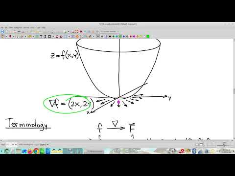
The gradient of a real-valued function assigns a vector to each point, so the gradient can be viewed as a vector field rather than computed one point at a time.
At different points, the gradient generally has different vectors, just as any other vector field does.
Clark Bray Math identifies the gradient as an especially important vector field for later vector-calculus topics.

14:00 Anti-Gradients, Potential Functions, and the Physics Minus Sign

An anti-gradient is a scalar function whose gradient gives a specified vector field, reversing the operation of taking a gradient.
“Potential function” is the more common name for this scalar function, while Clark Bray Math prefers “anti-gradient” because it makes the inverse relationship explicit.
For a force field, the anti-gradient is the negative of potential energy: forces point toward decreasing potential energy, as gravity pulls downward.
The minus sign matters; omitting it reverses the physical relationship between force and potential energy.

18:00 Vector Fields for Fluids, Migration, and Anti-Gradient Limits

Fluid velocity fields describe air conditioning flow in a room, ocean currents, and the movement of pollutants through air or water.
Surface-water motion and animal migration can also be modeled with vector fields; herds of zebras or flocks of birds can be treated as collective flows.
Unlike the familiar single-variable case, many continuous vector fields do not have an anti-gradient; the geometric reasons become a major topic in chapter 6.
A vector field in two dimensions must assign two output components to each input point, unlike a scalar function such as x².

22:55 Deriving Flux as Volume Flow Through an Oriented Surface

Flux measures fluid volume per unit time passing through a surface, in units such as cubic meters per second; it is distinct from particle velocity in meters per second.
For a small surface area A with unit normal n, the fluid’s displacement over a short time is its velocity multiplied by the time interval.
Only the displacement component perpendicular to the surface contributes to the volume crossing it, so the flow rate is the velocity field dotted with n and multiplied by A.
The fishing-net example illustrates why both net area and orientation matter: a horizontal net may intercept little flow even when the current is strong.

31:47 Mass Flux: Incorporating Density into the Vector Field

When the desired quantity is mass per unit time rather than volume per unit time, mass is computed as density multiplied by volume.
Representing a flow with the vector field density times velocity makes the same flux calculation yield mass flow through the surface.
The density factor is useful when tracking quantities such as kilograms of fluid or the number of animals moving through a region.
Flux therefore applies beyond volume transport when the vector field includes the relevant density.

35:15 Flow Lines as Particle Paths in a Velocity Field

A flow line describes the path of a particle carried along by a fluid, such as a leaf moving with a river current.
The governing equation states that the particle’s velocity equals the vector field evaluated at its current position: position derivative = F(position).
In coordinates, a three-dimensional field with components F₁, F₂, and F₃ gives the system x′ = F₁, y′ = F₂, z′ = F₃.
For F(x, y) = (-y, x), the unit-circle parameterization x = cos t, y = sin t satisfies the equations and traces the circulating path.

41:22 Use Both Force and Fluid Interpretations of Vector Fields

Force fields and fluid-flow fields are complementary ways to interpret vector fields; neither perspective replaces the other.
Electromagnetism requires force-based reasoning for some ideas and fluid-based reasoning for others.
Clark Bray Math recommends practicing both interpretations early rather than ignoring fluids or forces based on personal preference.

43:22 The Del Operator and Divergence as Local Outflow

The del operator, written ∇, produces the gradient when applied to a scalar function; ∇ is the operator, while ∇f is the resulting gradient.
Applying the dot product of ∇ with a vector field gives its divergence, written ∇ · F or div F, by differentiating corresponding field components and adding the results.
Positive divergence is introduced as a qualitative measure of fluid flowing outward from the point where it is computed.
Outward flow can represent material leaving a region and reducing its local density, or a source generating material; light bulbs provide an example of photons flowing outward.
Chapter 7 develops the interpretation further, including cases that combine generation and depletion rather than fitting only one extreme.

Summary, takeaways, and chapters were generated by AI from the video's transcript and may contain errors. The video belongs to its creator, Clark Bray Math.