2026 09 28 Math219 01

Overview

Clark Bray Math derives the geometric meaning of the gradient: at a point, it points in the direction of greatest increase, and its magnitude is the maximum directional derivative. The lecture then shows that gradients are normal to level sets and uses that fact to find tangent planes, before motivating the implicit function theorem with the need to verify that a dependent variable is locally a function.

Key takeaways

At a point where the gradient is nonzero, the unit gradient gives the direction of fastest increase, while the gradient’s magnitude is the maximum directional derivative over all unit directions.
For a differentiable function, the gradient is orthogonal to every tangent direction of its level set because the function’s directional derivative along that set is zero.
To use a gradient as a normal to a surface, first express the surface as a level set and take the gradient of the function defining that level set.
Implicit differentiation of a relation such as x² + y² = 1 requires establishing that y is locally a function of x; a vertical tangent prevents that representation.
The implicit function theorem gives a practical local test: to solve for a chosen variable, the partial derivative with respect to that variable must be nonzero at the point.

Chapters

0:00 Directional Derivatives and the Fastest-Increase Question

A directional derivative extends a partial derivative from standard basis directions to any unit-vector direction.
Using temperature across a location-based domain, the lecture asks which direction makes the function increase fastest.
The same optimization question applies to quantities such as engine efficiency or business profit as design parameters change.

6:40 Maximizing the Directional Derivative with a Dot Product

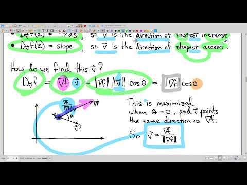
The directional derivative in a unit direction v is the dot product of the gradient at the point and v.
While comparing directions at a fixed point, the gradient is constant; the only changing factor is the angle between it and v.
The dot-product formula is largest when the angle is zero, so the maximizing direction is the unit vector pointing along the gradient.

12:00 Gradient Magnitude, Steepest Ascent, and the Hill Example

Substituting the unit gradient direction into the directional-derivative formula gives the gradient’s magnitude as the maximum rate of increase.
The gradient therefore has a geometric interpretation: its direction is fastest increase, and its magnitude is the rate of increase per unit distance.
At the illustrated point above (1, 3), the gradient has magnitude 2√2 and points southwest, indicating the direction of steepest ascent on the hill.
A point in the graph in R³ is distinct from its input location in the domain R²; compute the gradient using the domain coordinates.

21:00 Why Gradients Are Orthogonal to Level Sets

A function has a constant value along any curve contained in one of its level sets.
The velocity vector of motion along that curve is tangent to the level set, and the directional derivative in that tangent direction is zero.
Because the directional derivative equals the gradient’s dot product with the tangent vector, the gradient is orthogonal to every tangent vector of the level set.
The gradient can be the zero vector, so orthogonal is more precise than assuming a nonzero perpendicular vector.

27:40 Rewriting a Graph as a Level Set to Find a Normal

The level-set normal rule applies to a function’s level set, not to a picture or graph without first specifying its defining equation.
Rewrite a graph equation such as z = f(x, y) as an equation of the form g(x, y, z) = constant to express the same surface as a level set.
The relevant normal vector is the gradient of the same function whose level set describes the surface.
Horizontal contour lines of the original graph are not the same construction as rewriting that graph as a level set in three variables.

33:00 Using a Level-Set Gradient for a Tangent Plane

A tangent-plane equation requires a point on the plane and a normal vector.
For a surface given by an equation in x, y, and z, move terms to rewrite it as a level set of a function.
Evaluate that function’s gradient at the specified point to obtain a normal vector, then use it to form the tangent-plane equation.

36:50 Why Implicit Differentiation Requires a Function

Differentiating an equation such as x² + y² = 1 with respect to x and using the chain rule assumes that y is a function of x.
An implicit curve may fail the vertical line test globally, so a single x-value can correspond to multiple y-values.
Derivatives apply to functions; treating y as a function without establishing that relationship makes the differentiation argument unjustified.
Restricting attention to a small neighborhood can make y a local function of x when the curve is not vertical there.

42:30 Local Functions Fail at Vertical Tangents

At a point with a vertical tangent, narrowing the neighborhood does not make the curve pass the vertical line test.
When y cannot be represented as a function of x even locally, dy/dx is not defined by that function-based argument.
The lecture identifies a vertical tangent as the geometric source of the curve wrapping under itself and causing the local function problem.

45:00 The Implicit Function Theorem’s Nonzero Partial Test

For a curve described as a level set F(x, y) = C, a vertical tangent corresponds to a horizontal gradient and therefore F_y = 0.
If F_y is nonzero at a point, the implicit function theorem guarantees that y can be treated as a function of x in a neighborhood of that point.
In the illustrated example, F_y = 2y, so the local-function condition requires y ≠ 0; the problematic points lie on the x-axis.

48:10 Generalizing the Implicit Function Test to Any Variable

For a level-set surface in three dimensions, a surface folding so that z cannot be locally determined by x and y is associated with F_z = 0.
To solve locally for a chosen variable, check that the partial derivative with respect to that variable is nonzero at the point.
The implicit function theorem extends this criterion to appropriately smooth functions and surfaces in any dimension.

Summary, takeaways, and chapters were generated by AI from the video's transcript and may contain errors. The video belongs to its creator, Clark Bray Math.