2026 09 23 Math219 03

Overview

Clark Bray Math develops practical methods for applying the multivariable chain rule: distinguish input and output variables, use dependency diagrams, and introduce an identity variable when dependencies do not form a direct composition. The lecture extends these methods to second derivatives in polar coordinates and shows how changing coordinates makes the Laplacian of a radial potential, such as 1/r, far easier to compute in spherical coordinates than in rectangular coordinates.

Key takeaways

Rename intermediate outputs in a composition—such as using y for the output of f—so each variable has one role and the chain rule’s evaluation points remain clear.
The standard chain rule requires matching stages: when a downstream function also depends directly on an original input, an identity variable such as x₁*=x₁ can create a valid composition.
A dependency diagram should represent actual functional dependencies, including newly formed derivatives like zₓ and zᵧ when they appear in second-derivative calculations.
For z=z(x,y) with x=r cos θ and y=r sin θ, the diagram shows that θ is constant during an r-partial, allowing factors such as cos θ to be treated as constants.
C² smoothness justifies interchanging mixed partials, so zₓᵧ=zᵧₓ in the polar-coordinate second-derivative example.
Coordinate choice can turn a long calculation into a short one: the spherical Laplacian of a radial 1/r potential is zero because both angular terms vanish and the radial expression reduces to a constant before its final derivative.

Chapters

0:00 Single-Variable Chain Rule: Rename the Intermediate Output

For a composition such as f(x)=x² followed by g(y)=y³, g′ must be evaluated at f(x), not at x.
Treat the variable in a function’s formula as a dummy placeholder: rename g’s input from x to y because y is the output of f.
The renamed-variable setup yields the correct derivative 3(x²)²·2x=6x⁵ without mentally reusing x for different roles.

6:40 Multivariable Compositions: Label Inputs and Outputs Separately

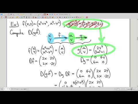
When f takes x and y to produce outputs, label those outputs u and v, then rewrite the next function g as a function of u and v.
A dependency diagram records which variables enter each function and which variables emerge from it.
Variable names such as u,v or s,t are choices rather than fixed conventions; the essential rule is not to reuse an input name for an intermediate output.

11:20 Why Some Dependency Diagrams Are Not Function Compositions

The ordinary chain rule applies to compositions where every output of the first function is exactly an input to the next.
In a dependency network where z₁ depends on y₁, y₂, and directly on x₁, its inputs do not match the outputs of the preceding stage.
Writing ∂z₁/∂x₁ can then be ambiguous: it might mean varying x₁ while holding y₁,y₂ fixed or differentiating the fully composed function.

16:28 Use an Identity Variable to Make the Chain Rule Apply

Insert a new intermediate variable x₁* defined by x₁*=x₁, placing it between the original inputs and the dependent variables.
Rewrite the downstream function using x₁* in place of its direct x₁ input; the value is unchanged, but the stages now form a composition.
For ∂z₁/∂x₁, sum one chain-rule term for each intermediate variable, including the newly introduced x₁*.

21:11 Set Up Polar-Coordinate Second Derivatives with a Diagram

Assume z is a C² function of x and y, with x=r cos θ and y=r sin θ.
The first derivative zᵣ follows two dependency paths, through x and through y; compact notation such as zₓ means ∂z/∂x.
For second derivatives, expect to differentiate products; whether a factor is constant depends on the variable being differentiated.

26:33 Extend the Dependency Diagram for Derivatives of Derivatives

The expression zₓ is not a function of both (x,y) and (r,θ) simultaneously; it is a function of x and y.
Add zₓ and zᵧ to the diagram as functions of x,y, then apply the chain rule to their r-derivatives through x and y.
When differentiating zₓ cos θ with respect to r, θ is constant, so cos θ factors out; the diagram makes this dependency clear.

33:03 Simplify Second-Partials Carefully and Use C² Smoothness

Mixed second partials such as zₓᵧ and zᵧₓ are equal here because z is assumed to be C².
A diagram needs new entries when a derivative such as zₓ becomes a function in a later chain-rule step, but not for every algebraic expression built from existing entries.
For long derivative expansions, use large parentheses and align terms vertically to make product-rule steps and algebra checks easier.

40:09 The Laplacian and Its Spherical-Coordinate Form

The Laplacian is the sum of the three unmixed second partials in rectangular coordinates and appears in models of waves, heat conduction, and electric or gravitational fields.
The spherical-coordinate Laplacian looks more elaborate, but it represents the same operator after applying the chain rule to the coordinate transformation.
Differential-operator notation can omit the function being acted on when the goal is to describe the operation itself.

43:40 Convert Polar Derivative Operators with a 2×2 System

In polar coordinates, the r- and θ-derivative operators can be written in terms of the rectangular x- and y-derivatives using the chain rule.
Solve the resulting pair of operator equations as a 2×2 simultaneous system to express rectangular partial derivatives in terms of polar partial derivatives.
Clark Bray Math notes these conversion formulas are useful for a future exam equation sheet, though the current lecture’s material is not on Friday’s exam.

48:42 A Radial Potential Makes the Spherical Laplacian Simple

For the radial potential 1/r, the spherical Laplacian’s angular derivatives vanish because the function contains neither θ nor φ.
In the radial term, differentiating 1/r gives −1/r²; multiplying by r² produces a constant, whose next derivative is zero.
The same harmonic-function check is cumbersome in rectangular coordinates, where the equivalent expression involves √(x²+y²+z²), illustrating when spherical coordinates simplify the work.

Summary, takeaways, and chapters were generated by AI from the video's transcript and may contain errors. The video belongs to its creator, Clark Bray Math.