2026 09 18 Math219 03

Overview

Clark Bray Math develops the derivative as a linear map from input changes to output changes, then connects that view to gradients, second partial derivatives, and parametric motion. The lecture interprets a parametric curve’s derivative as its velocity, explains when mixed partials can be reordered, and emphasizes that an integration constant must be solved from an initial condition rather than assumed to equal it.

Key takeaways

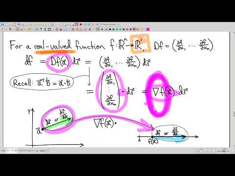
A multivariable derivative is a matrix that linearly maps small input changes to corresponding output changes; for a real-valued function, the same action is a dot product with the gradient.
When a function has the required continuous partial derivatives, mixed partial derivatives can be reordered; smooth combinations of polynomials, trigonometric functions, and exponentials satisfy this condition at every order.
Second partial derivatives describe curvature along chosen directions, so a surface can curve upward in one direction and downward in another at the same point.
The derivative of a position-valued parametric curve is its velocity vector: its direction gives the direction of motion and its magnitude gives speed.
An integration constant is determined by applying the initial condition to the entire antiderivative expression; it is not generally equal to the initial position itself.
Time derivatives of vector dot products and cross products obey product rules, which are useful when differentiating vector-valued quantities in physics.

Chapters

0:00 Derivative Matrices Map Input Changes to Output Changes

The derivative matrix (also called the Jacobian matrix) is the linear transformation in the linear approximation that turns differential input changes into corresponding output changes.
A function maps points in its domain to points in its target; its derivative maps changes in the domain to changes in the target.
Dividing input and output changes by time gives the related velocity interpretation: the derivative maps an input velocity to an output velocity.

8:04 A Real-Valued Derivative Matrix Is the Gradient

For a real-valued function, the derivative matrix has one row, so its matrix-vector product can be written as a dot product with the gradient.
The gradient is the transpose of that single-row derivative matrix and has geometric properties such as direction and magnitude.
The discrete-change interpretation involves linear approximation, while the velocity mapping along motion gives the exact output velocity.

11:35 Differentiation Is Linear and Mixed Partials Can Commute

Differentiation is linear: the derivative of a linear combination of functions is the same linear combination of their derivatives.
Higher partial derivatives are obtained by taking partial derivatives repeatedly, just as a second derivative is the derivative of a first derivative.
Mixed partials can be reordered when the relevant partial derivatives exist and are continuous; functions built from polynomials, sines, cosines, and exponentials are typically C-infinity.

18:22 Unmixed Second Partials Reveal Saddle-Shaped Curvature

For fxx, y remains constant throughout both differentiations, so the second partial is the ordinary second derivative of an x-direction cross-section.
For fyy, x remains constant, and the curvature of the y-direction cross-section determines the sign of the second partial.
A saddle surface can be concave down in one direction and concave up in another at the same point, unlike a one-variable curve.

22:37 Reading a Mixed Partial as Changing Cross-Section Slopes

For an x partial of the y partial, the first derivative measures slopes along y-direction cross-sections of the graph z = f(x,y).
The second derivative measures how those y-direction slopes change as x changes; increasing slopes across x indicate a positive mixed partial.
The geometric interpretation involves a twist in the surface, and reversing the order examines the other family of cross-sections.

30:24 Parametric-Curve Derivatives Are Tangent Vectors

A parametric curve gives position as a function of one parameter, often time, so its derivative matrix has a single column.
The difference quotient uses a vector displacement between positions, unlike the scalar change in y used for a single-variable graph.
Taking the limit produces a tangent vector pointing in the curve’s direction of motion, not a tangent-line slope.

38:35 Velocity Is the Derivative of a Parametric Curve

The tangent vector’s magnitude is the limit of distance traveled divided by elapsed time, giving the curve’s speed.
Together, direction of motion and speed identify the parametric curve’s derivative as its velocity; differentiating velocity gives acceleration.
An optional geometric argument uses motion around the unit circle to derive sine and cosine derivative formulas from the velocity interpretation.

41:13 Integrating Velocity and Solving for the Integration Constant

Acceleration is the derivative of velocity, while position is found by taking an antiderivative of velocity and adding an integration constant.
The constant is not automatically the initial condition: substitute the initial time into the position equation and solve for the constant using the given initial position.
Clark Bray Math stresses fluency with substitutions, integration by parts, and trigonometric substitutions, noting their relevance to engineering problems involving circles.

46:39 Vector Product Rules and the Kepler Material Exception

Most of the section on Kepler’s laws is omitted for course pacing, but Proposition 1.4 remains assigned for its product rules.
The time derivative of a dot product or cross product follows the expected product rule, with a derivative applied to each vector factor in turn.
The class ends after the vector-product rule discussion, with the remaining Kepler-related material largely excluded.

Summary, takeaways, and chapters were generated by AI from the video's transcript and may contain errors. The video belongs to its creator, Clark Bray Math.