2026 09 18 Math219 02

Overview

Clark Bray develops a geometric interpretation of mixed second partials as surface twist, then connects derivatives of parametric curves to velocity and speed. He uses derivatives as multiplicative factors to derive the multivariable chain rule, emphasizing Jacobian dimensions, evaluation points, and the importance of matrix order.

Key takeaways

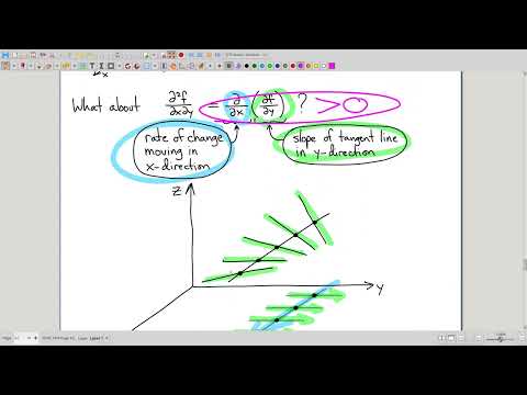
A mixed partial such as fₓᵧ measures how the y-direction tangent slopes change as x changes; increasing slopes correspond to a positive surface twist.
For a parametric curve, the derivative vector is velocity: it points along the curve, and its magnitude is speed.
The unit-circle parametrization (cos t, sin t) has unit speed, and rotating its position vector by 90 degrees yields velocity coordinates that establish the sine and cosine derivative formulas.
An integration constant must be found by applying the initial condition to the integrated expression; it does not generally equal the initial position.
For a composition z = g(f(x)), the multivariable chain rule is Dg(f(a))Df(a), with Jacobian dimensions determining whether the matrix product is valid.
Jacobian multiplication is order-sensitive, so chain-rule calculations should follow the sequence of function actions and evaluate each derivative at the point where its function acts.

Chapters

0:00 Mixed Second Partials Measure How Cross-Section Slopes Change

Unmixed second partials such as fₓₓ correspond to concavity along a single coordinate direction.
For fₓᵧ, track tangent-line slopes in the y direction while moving through x; increasing slopes indicate a positive mixed partial.
A positive mixed partial can be visualized as a twist, or torsion, in the surface rather than ordinary single-variable concavity.

8:47 Course Roadmap: Chapter 3 Before Section 2.5

Clark Bray’s class sequence moves from section 2.4 to section 3.1, then returns to section 2.5.
The course website has a book-order content syllabus and a reordered class-specific syllabus; green topics on the schedule are exam material.
Exams allow a one-page notes sheet, though older exam copies may still say that notes are prohibited.

11:33 Parametric-Curve Derivatives Are Velocity Vectors

A parametric curve has one input parameter, so its derivative matrix has one column and its partial derivatives reduce to ordinary single-variable derivatives.
The derivative vector points tangent to the curve and its magnitude is distance traveled per unit time, or speed.
The derivative of position is velocity; differentiating velocity gives acceleration.

18:25 Deriving Sine and Cosine Derivatives from Unit-Circle Motion

The curve (cos t, sin t) traces the unit circle at speed 1.
Its velocity is tangent to the circle, has magnitude 1, and is the position vector rotated by 90 degrees.
Reading the velocity coordinates gives d(cos t)/dt = −sin t and d(sin t)/dt = cos t without a limit calculation.

25:00 Recovering Position from Velocity and Solving for the Constant

Position can be found by integrating velocity, while acceleration is the derivative of velocity.
The course assumes fluency with integration by parts, substitution, and trigonometric substitution; Clark Bray notes that circle-related applications make trig substitutions especially useful for engineers.
Determine an integration constant by substituting the initial time and position into the integrated expression; in the example, r(0) = 56 and the expression contributes 31, so the constant is 25—not the initial value.

30:12 Vector-Valued Product Rules and the Kepler-Section Exception

Planetary-motion material and Kepler’s laws at the end of section 3.1 are excluded because they are not needed for the course’s vector-calculus path.
The required result is proposition 1.4: derivatives of dot products and cross products of vector-valued functions follow the expected product-rule pattern.
The product rules apply to vector-valued functions such as position or velocity, not only scalar functions.

32:05 Single-Variable Chain Rule as Multiplication of Derivative Factors

For a composition x → f(x) = y → g(y) = z, the output of f becomes the input of g.
Interpret each derivative as a factor relating input velocity to output velocity; the overall factor is the product of the two derivatives.
The resulting principle is that differentiation turns composition into product, yielding the single-variable chain rule.

39:35 The Multivariable Chain Rule Composes Jacobian Matrices

In multiple dimensions, input and output velocities are vectors, so the derivative factor relating them is a Jacobian matrix.
For z = g(f(x)), the Jacobian factors compose as Dg(f(a))Df(a): the inner function’s derivative acts first, followed by the outer function’s derivative.
The rule works across different dimensions, provided the Jacobian sizes match—for example, mappings from 17 dimensions to 5 and then to 31.

45:23 Track Evaluation Points and Matrix Order Carefully

The outer derivative Dg is evaluated at f(a), the point where g receives its input; the inner derivative Df is evaluated at a.
Unlike scalar multiplication in the single-variable chain rule, matrix multiplication is not commutative, so reversing Jacobian order changes the result.
To avoid notation errors across composition symbols, diagrams, and matrices, track which function acts first and which acts second rather than relying on left-versus-right wording.

Summary, takeaways, and chapters were generated by AI from the video's transcript and may contain errors. The video belongs to its creator, Clark Bray Math.