2026 09 18 Math219 01

Overview

Clark Bray Math connects derivatives of parametric curves to velocity, then uses the idea that derivatives act as multiplicative factors to motivate the multivariable chain rule. The class derives the sine and cosine derivatives geometrically, reviews coordinate-by-coordinate integration and integration constants, and emphasizes that chain-rule matrix order and evaluation points matter.

Key takeaways

For a parametric curve r(t), r′(t) is a velocity vector: its direction is tangent to the motion and its magnitude is speed.
The unit-circle parameterization r(t) = (cos t, sin t) has tangent velocity (−sin t, cos t), providing a geometric derivation of both basic trigonometric derivative formulas.
When integrating a vector-valued velocity, integrate each coordinate separately and use the initial position to solve for the integration constant; the constant is not generally the initial position itself.
The multivariable chain rule is D(g ∘ f)(a) = Dg(f(a))Df(a): the inner function’s derivative acts first, so its matrix appears on the right.
In a derivative matrix, output variables correspond to rows and input variables to columns; therefore ∂z₃/∂x₁ is found in row 3, column 1.

Chapters

0:00 Parametric-Curve Derivatives Are Vectors, Not Graph Slopes

For a parametric curve with one input parameter t, each coordinate’s partial derivative is an ordinary single-variable derivative.
The derivative is the limit of vector secant displacements divided by elapsed time; unlike a graph’s rise-over-run, its numerator is a vector.
The resulting tangent vector points in the direction of motion, and its magnitude is speed, so it represents velocity.

6:09 A Derivative Matrix for One Parameter Acts Like a Velocity Vector

A derivative matrix for a curve with one input has a single column, so its algebraic action matches that of a vector.
Clark Bray Math distinguishes the general derivative matrix, which may have multiple columns, from the one-column case used for a parametric curve.
Writing the curve in coordinates or as a linear combination of coordinate-direction vectors gives the same componentwise derivative.

10:40 Unit-Circle Geometry Derives the Sine and Cosine Derivatives

The unit-circle parameterization has position vector (cos t, sin t), with speed 1 and a tangent velocity vector.
Perpendicular radius and tangent directions, along with congruent triangles, identify the velocity components as (−sin t, cos t).
Matching velocity to the derivative of position yields d(cos t)/dt = −sin t and d(sin t)/dt = cos t without a limit calculation.

16:15 Recovering Position from Velocity and Handling the Integration Constant

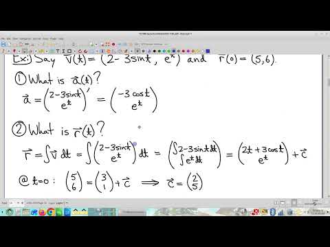
Acceleration is found by differentiating velocity, while position is recovered by integrating each velocity coordinate separately.
Clark Bray Math expects foundational single-variable integration techniques, including basic substitutions, integration by parts, and trigonometric substitutions.
An initial position determines the integration constant by substitution; the constant is not generally equal to the initial position.
The common misconception arises in polynomial examples whose integrated terms all contain t and therefore vanish at t = 0.

21:49 Vector-Valued Product Rules and the Dot Product

Kepler’s historical planetary-motion calculations are treated as optional because they are not essential prerequisite material for the course.
The derivative of the dot product of two vector-valued functions follows the familiar product-rule pattern.
The class treats the dot-product rule as a core fact to know, while setting aside the less essential historical calculations.

23:41 Single-Variable Chain Rule: Derivatives as Multiplicative Factors

Clark Bray Math frames a derivative as the factor that converts input velocity into output velocity.
For a composition x → f(x) → g(f(x)), f′ maps x-velocity to y-velocity and g′ maps y-velocity to z-velocity.
Because successive factors multiply, the derivative of a composition is the product of the component derivatives.
The evaluation points follow the function domains: f′ is evaluated at a, while g′ is evaluated at f(a).

32:20 Extending the Chain Rule to Multivariable Derivative Matrices

In multiple dimensions, the derivative matrix is the factor that maps an input-velocity vector to an output-velocity vector.
For f followed by g, the composition’s derivative is Dg(f(a)) multiplied by Df(a), with the rightmost matrix acting first.
The argument works across any compatible positive-integer dimensions because the intermediate space determines matching matrix dimensions.
Differentiation turns a composition into a matrix product, extending the single-variable factor interpretation.

38:16 Composition Order, Matrix Order, and Evaluation Points

Although f acts first in the diagram, f appears on the right in g ∘ f and in the derivative matrix product.
The derivative of g must be evaluated at f(a), the point in g’s domain reached after applying f.
Reversing matrix order can produce a wrong answer even when both matrices are square and multiplication is dimensionally allowed.
Clark Bray Math recounts losing a month of graduate work to an analogous ordering error and urges checking the action order.

42:14 Applying the Multivariable Chain Rule and Reading a Jacobian Entry

The worked example composes f from two x-variables to three y-variables with g from three y-variables to three z-variables.
The given data provide Df(1, 2) and Dg(f(1, 2)); identifying f(1, 2) as (3, 1, 0) supplies the correct evaluation point.
The composition derivative is computed as Dg(f(1, 2)) Df(1, 2), with matrix order checked before multiplication.
To extract ∂z₃/∂x₁, select row 3 for output z₃ and column 1 for input x₁; the example’s entry is 3.

Summary, takeaways, and chapters were generated by AI from the video's transcript and may contain errors. The video belongs to its creator, Clark Bray Math.