2026 09 16 Math219 03

Overview

Clark Bray Math develops the multivariable linear approximation from the requirement that it match a function’s value and derivatives at a base point. For vector-valued functions, the derivative is the Jacobian matrix, which maps input changes to estimated output changes; continuous partial derivatives provide a practical sufficient condition for the linear approximation to work.

Key takeaways

For a scalar-valued function, the linear approximation at a is f(a) + ∇f(a) · (x − a), with the gradient collecting all input-variable partial derivatives.
For a function from ℝⁿ to ℝᵐ, the Jacobian has m output rows and n input columns, and the approximation is f(a) + Df(a)(x − a).
Having every partial derivative at a point does not by itself guarantee a valid linear approximation; the example z = r sin(3θ) has coordinate-axis partials at the origin but behaves irregularly in other directions.
Continuous partial derivatives guarantee differentiability, making continuous differentiability a practical sufficient test for whether linear approximations work.
Differentiability implies continuity, so discontinuity is enough to rule out differentiability; the converse implication does not generally hold.
The multivariable derivative is a linear map from input changes to output changes, represented by the Jacobian matrix rather than by a single scalar.

Chapters

0:00 Extending Single-Variable Linearization to Several Inputs

A linear approximation at a base point a should match the function’s value and derivative at a.
For a real-valued function of several variables, matching derivatives means matching every partial derivative at the base point.
To verify the approximation, differentiate its formula with respect to each input variable, treating quantities evaluated at a as constants.

5:07 The Gradient Turns Scalar Linearization into a Dot Product

The linear terms pair each partial derivative of f with the corresponding coordinate of x − a.
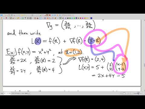
Defining the gradient as the vector of partial derivatives rewrites the scalar-valued approximation as f(a) + ∇f(a) · (x − a).
In the example based at (1, 2), the approximation is assembled from f(1, 2), the gradient at (1, 2), and the displacement from (1, 2).

11:26 Vector-Valued Linear Approximation Uses a Derivative Matrix

For a function with multiple outputs, the approximation has the form f(a) + Df(a)(x − a).
The matrix Df contains the partial derivatives of every output coordinate with respect to every input variable.
The approximation must match the values and all input-variable partial derivatives of every output coordinate.

17:29 Reading Jacobian Rows, Columns, and Dimensions

Each row of Df contains the partial derivatives of one output coordinate, such as f₁ or fₘ.
Each column contains derivatives with respect to one input variable, such as x₁ or xₙ; rows are outputs and columns are inputs.
For a function from ℝⁿ to ℝᵐ, Df has m rows and n columns, so transposing it can make the matrix product invalid or silently wrong when it is square.
Evaluating f(a) for a vector-valued function correctly produces a vector, because the function’s outputs are vectors.

22:09 A Linear Approximation’s Graph Is a Tangent Line or Plane

In single-variable calculus, the graph of the linear approximation is the tangent line; the function and its graph are distinct objects.
For a real-valued function of two variables, the graph of its linear approximation is the tangent plane.
The tangent plane follows the surface locally when a valid linear approximation exists.

25:14 Why Partial Derivatives Alone Can Miss a Differentiability Failure

Multivariable differentiability is more subtle than having partial derivatives, because infinitely many directions combine the input coordinates.
The example z = r sin(3θ) has well-behaved partial derivatives along the coordinate axes at the origin, yet its graph has a fold-like irregularity there.
An approximation inferred from those partial derivatives can fail badly in other directions, showing that partial derivatives alone do not guarantee a good linear approximation.

35:50 Continuous Partial Derivatives Provide a Practical Differentiability Test

A function is continuously differentiable when its partial derivatives exist and are continuous.
The theorem used in class says continuous differentiability guarantees differentiability, avoiding a direct check of the more demanding definition.
For a polynomial, the partial derivatives are also polynomials and are continuous everywhere, so the function is differentiable everywhere.

41:47 Differentiability Implies Continuity, but Not Conversely

The implication “differentiable implies continuous” also holds for multivariable functions.
Its contrapositive shows that a discontinuous function cannot be differentiable.
Continuous differentiability is a convenient sufficient test, but some differentiable functions do not have continuous partial derivatives.

43:40 The Differential Estimates Change from Base Point to Nearby Point

Rearranging the linear approximation gives Df(a)(x − a) as the predicted change in the output.
The displacement x − a is the input change, while the change in the linear approximation estimates how much f changes.
A differential is a linear estimate of change, connecting the multivariable construction to the familiar single-variable idea.

47:21 The Jacobian Matrix Is the Multivariable Derivative

For vector-valued functions, input and output changes are vectors, so the derivative must map vectors to vectors.
The matrix Df performs that mapping, which is why it—not an individual partial derivative—is the derivative in the general multivariable setting.
Single-variable derivatives being scalar-valued is a special case; the broader derivative concept is a linear map represented by a matrix.

Summary, takeaways, and chapters were generated by AI from the video's transcript and may contain errors. The video belongs to its creator, Clark Bray Math.