10 First-Order Differential Equations to Master Before Your Exam

Overview

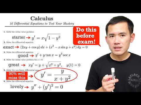
blackpenredpen works through 10 first-order differential-equation problems, demonstrating separable, exact, Bernoulli, homogeneous, linear-after-inversion, Clairaut, almost-exact, and Riccati methods, plus substitutions that reduce equations involving higher derivatives. The examples emphasize checking for solutions lost through division, using initial conditions carefully, and recognizing nonuniqueness and singular solutions.

Key takeaways

For separable equations, dividing by an expression involving y can remove equilibrium solutions: y′ = x√(1 − y²) requires checking y = ±1 separately, and the initial value y(0) = −1 admits the constant solution y = −1.
An equation M dx + N dy = 0 is exact when Mᵧ = Nₓ; integrating one component and matching the other recovers a potential function defined implicitly as F(x,y) = C.
Bernoulli equations y′ + P(x)y = Q(x)yⁿ become linear under u = y^(1−n); for n = 3, u = y⁻², but solutions excluded by division by y must still be tested.
Homogeneous equations involving y/x can be reduced with u = y/x, while equations easier to solve for x can be inverted; both strategies expose separable or linear structure hidden in the original form.
Recognizing derivative patterns reduces higher-order equations: y y″ + (y′)² = (yy′)′, and substituting u = y′ in y″ + (y′)² = 0 produces a separable equation.
Clairaut’s equation y = xy′ + (y′)² has both a one-parameter family y = Cx + C² and a singular envelope y = −x²/4; Riccati equations can similarly be reduced when a particular solution is supplied.

Chapters

0:00 Ten First-Order Differential Equations: Methods and Exam Goals

The set covers separable, linear, exact, almost-exact, Bernoulli, homogeneous, Clairaut, and Riccati equations.
Substitution is also used to reduce equations whose original form does not match a standard first-order type.

0:44 Problem 1: Separate Variables in y′ = x√(1 − y²)

Rearrange to dy/√(1 − y²) = x dx and integrate to obtain arcsin(y) = x²/2 + C.
Apply the inverse sine to express the nonconstant solution family and use the initial condition to select a branch.

3:03 Problem 1: Check Boundary Equilibria and Nonuniqueness

Dividing by √(1 − y²) excludes the equilibrium solutions y = 1 and y = −1, so they must be checked separately.
For the stated initial value y(0) = −1, the constant solution y = −1 is also valid, illustrating nonuniqueness.

5:44 Problem 2: Verify Exactness with Mixed Partial Derivatives

Write M = 2xy + cos(y) and N = x² − x sin(y) + eʸ in M dx + N dy = 0.
Since Mᵧ = 2x − sin(y) and Nₓ = 2x − sin(y), the equation is exact.

9:13 Problem 2: Build the Potential Function

Integrate M with respect to x to get F(x,y) = x²y + x cos(y) + g(y).
Matching Fᵧ to N gives g′(y) = eʸ, so the implicit solution is x²y + x cos(y) + eʸ = C.

14:13 Problem 3: Convert the Bernoulli Equation with u = y⁻²

Recognize y′ + y tan(x) = y³ sec(x) as a Bernoulli equation with exponent n = 3.
Set u = y^(1−3) = y⁻²; dividing by y³ and differentiating the substitution produces u′ − 2 tan(x)u = −2 sec(x).

17:49 Problem 3: Use an Integrating Factor and Restore the y Solutions

The linear equation in u has integrating factor cos²(x), turning its left side into the derivative of cos²(x)u.
Integration gives cos²(x)y⁻² = −2 sin(x) + C; y = 0 must also be checked because the original equation was divided by y³.

25:05 Problem 4: Recognize a Homogeneous Equation with y/x

For x y′ = y + √(x² + y²), assume x > 0 and divide by x to expose the ratio y/x.
Set u = y/x, or y = xu; then y′ = xu′ + u and the equation reduces to xu′ = √(1 + u²).

35:03 Problem 5: Reverse the Dependent and Independent Variables

For y′ = y/(x + y²), treat x as a function of y and use dx/dy = (x + y²)/y.
The resulting linear equation, dx/dy − x/y = y, has integrating factor 1/y and yields x = y² + Cy.
Check y = 0 separately because the variable reversal divides by y; the constant-zero solution satisfies the original equation where defined.

42:35 Problem 6: Reduce y″ + (y′)² = 0 by Setting u = y′

With u = y′, the equation becomes u′ = −u², a separable first-order equation.
For u ≠ 0, integration gives y′ = 1/(x + C₁), then y = ln|x + C₁| + C₂.
The division by u omits u = 0, which supplies the additional constant solutions y = C.

47:49 Problem 7: Solve Clairaut’s Equation and Find Its Envelope

Identify y = xy′ + (y′)² as Clairaut’s equation and set p = y′.
Differentiating y = xp + p² gives (x + 2p)p′ = 0, creating two solution cases.
The case p = C gives y = Cx + C²; x + 2p = 0 gives the singular solution y = −x²/4.

54:31 Problem 8: Integrate the Product Derivative in y y″ + (y′)² = 1

Recognize y y″ + (y′)² as the derivative of yy′, reducing the equation to (yy′)′ = 1.
Integrate twice to obtain y² = x² + 2C₁x + 2C₂, with two constants because the original equation is second order.

58:37 Problem 9: Find an Integrating Factor for an Almost-Exact Equation

For the equation written as M dx + N dy = 0, compare Mᵧ and Nₓ; their mismatch shows it is not exact.
Evaluate (Nₓ − Mᵧ)/M; the expression simplifies to −4/y, identifying an integrating factor that depends only on y.
Integrating −4/y gives μ(y) = y⁻⁴, which converts the equation into an exact differential equation.

1:05:48 Problem 9: Recover the Potential After Multiplying by y⁻⁴

After applying μ(y) = y⁻⁴, integrate the new M with respect to x to obtain F = x²eʸ + xy⁻³ + g(y).
Matching Fᵧ to the new N gives g′(y) = 0, so the implicit solution is x²eʸ + xy⁻³ = C.
Check y = 0 in the original equation because the integrating factor is undefined there; y = 0 is also a solution.

1:10:20 Problem 10: Solve the Riccati Equation Using a Known Particular Solution

The equation y′ = 4x² − (2/x)y + y²/x⁴ comes with the particular solution y₁ = x³.
Use y = x³ + 1/u; differentiating requires the chain-rule term −u′/u², which reduces the equation to u′ = −1/x⁴.
Integrate to get u = 1/(3x³) + C and substitute back, yielding y = x³ + 3x³/(1 + Cx³), with the constant renamed.

Summary, takeaways, and chapters were generated by AI from the video's transcript and may contain errors. The video belongs to its creator, blackpenredpen.