10:3 Pipe Flow - Major Losses, Minor Losses, Type I and II Systems

Overview

Derek Elsworth explains how to combine major pipe friction losses, minor fitting losses, and the energy equation to size a pump. After reviewing the Moody chart and loss coefficients, he works through a jet example: a 100 kg load implies a 10 m/s jet, giving Reynolds number 10^6, an estimated 16 m pump head, and approximately 16 kW of required power.

Key takeaways

For fully developed laminar flow in a circular pipe, the Darcy friction factor is 64/Re, so friction changes with Reynolds number.
In fully rough turbulent pipe flow, friction factor depends mainly on relative roughness ε/D rather than Reynolds number.
Major losses scale with fL/D, while local losses scale with the sum of fitting coefficients; both multiply the velocity head V²/2g.
A 10 m/s flow of water through a 0.01 m² area has a volumetric flow rate of 0.1 m³/s and a velocity head of approximately 5 m.
In the worked example, a 10 m pipe with f ≈ 0.01 and D = 0.1 m produces about 5 m of major loss; five fittings with K = 0.2 add about 5 m.
The example’s 1 m elevation rise, 5 m outlet velocity head, 5 m major loss, and 5 m minor loss require about 16 m of pump head and 16 kW of hydraulic power.

Chapters

0:00 Pipe-Flow Modeling and the Pump-Sizing Problem

Derek Elsworth frames pipe flow as a practical, formula-based engineering tool for estimating system requirements.
He connects pipe modeling to similitude: geometric ratios, Reynolds number, and Euler number must match between model and prototype.
The Moody chart provides experimentally calibrated friction data for pipe-flow calculations.

3:36 Energy Equation: Major and Minor Head Losses

The energy equation accounts for elevation, pressure, velocity head, pump or turbine work, and both major and minor losses.
Major pipe loss follows the Darcy–Weisbach form: hL = f(L/D)(V²/2g).
A fitting loss is represented by hL = K(V²/2g), using the average velocity in the relevant pipe.

9:00 Laminar Pipe Flow and the 64/Re Friction Factor

For fully developed laminar flow in a circular pipe, the velocity profile is parabolic, with zero velocity at the wall and a maximum at the center.
The Navier–Stokes solution gives the Darcy friction factor f = 64/Re.
The corresponding major head loss is hL = (64/Re)(L/D)(V²/2g).

12:06 Reading Laminar, Transition, and Turbulent Regions on the Moody Chart

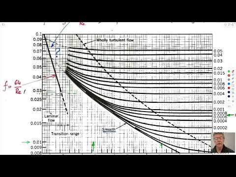
The Moody chart plots friction factor against Reynolds number on logarithmic axes and distinguishes laminar, transitional, and turbulent flow.
Laminar flow is associated with Reynolds numbers below roughly 2,000; the transition region leads into turbulent flow.
Pipe relative roughness, ε/D, separates the turbulent-flow curves, including the smooth-pipe curve.

17:00 Turbulent Flow, Roughness, and Velocity Profiles

In laminar flow, friction factor changes with Reynolds number; in fully rough turbulent flow, it is governed primarily by relative roughness.
Turbulent pipe flow has a flatter time-averaged velocity profile than the laminar parabolic profile, despite instantaneous eddies and fluctuations.
Elsworth uses a dye tracer in a tube to contrast orderly laminar motion with turbulent mixing.

22:03 Why Pipe Entries, Exits, and Bends Create Minor Losses

Minor losses arise from local flow changes such as contraction, expansion, separation, and turning at fittings.
Their head-loss form is hL = K(V²/2g); an exit into a large, stagnant tank has K = 1 because the pipe velocity is dissipated.
A gradual entry or larger bend radius can reduce separation and lower the loss coefficient.

27:10 How Bend, Tee, Thread, and Valve Geometry Changes K

A 45-degree bend generally produces less loss than a 90-degree bend, while a long-radius bend reduces loss compared with a tight turn.
Threaded connections can create more resistance than smooth flanged transitions because threads intrude into the flow.
T-junctions and valves have geometry- and flow-path-dependent loss coefficients; guide vanes can reduce separation in bends.

31:17 Setting Up the Jet Example and Pump-Head Calculation

The example models a jet lifting a 100 kg person or load, with a square pipe area of 0.01 m², equivalent to 0.1 m by 0.1 m.
Elsworth lays out the calculation chain: use momentum to find jet velocity, then Reynolds number, friction factor, head losses, pump head, and power.
The pipe route is assigned a total length of 10 m, a 1 m elevation rise, and five illustrative minor-loss elements.

38:00 Momentum Balance Gives a 10 m/s Jet Velocity

A control-volume momentum balance equates the load’s weight, approximately 100 kg × 10 m/s², to the jet’s momentum flux.
With water density 1,000 kg/m³ and area 0.01 m², the calculation gives a jet velocity of 10 m/s.
The energy-equation endpoints are both exposed to atmospheric pressure; the large upstream tank has negligible surface velocity.

43:03 Reynolds Number and the Pipe-Friction Loss Estimate

Using V = 10 m/s, characteristic diameter 0.1 m, water density 1,000 kg/m³, and viscosity 10⁻³ Pa·s gives Re ≈ 10⁶.
For a smooth pipe at that Reynolds number, the Moody chart supplies an estimated friction factor near 0.01.
With L = 10 m and D = 0.1 m, the major-loss multiplier fL/D is approximately 1, corresponding to about 5 m of head loss.

49:04 Adding Fitting Losses to Reach 16 m Pump Head and 16 kW

Five fittings at an illustrative K = 0.2 each give a total minor-loss coefficient of 1 and about 5 m of minor head loss.
The velocity head at 10 m/s is about 5 m; adding it to the 1 m elevation rise and 10 m of major-plus-minor losses yields a pump head of 16 m.
With water’s unit weight near 10,000 N/m³ and flow rate 0.1 m³/s, the estimated pump power is 16,000 W, or 16 kW—roughly 21 hp.

Summary, takeaways, and chapters were generated by AI from the video's transcript and may contain errors. The video belongs to its creator, Derek Elsworth.